I could say a lot about proper simulation of fMRI experiments. Basically it’s important to measure the efficiency of your design before an experiment (see here). If you wanted to perform the calculations yourself, MATLAB/Python/Octave are all options and the process is “fairly simple”.
Xmat = [design_matrix' * design_matrix];
main_effects(ct) = [ contrast' * (Xmat^-1) * contrast ];
But 1) if you don’t feel like writing your own code; 2) you want to test several designs to find the most efficient one, then you’re in luck. Today I’m mostly going to write about adjusting the stimulus timing files to find the most “efficient” design possible. When simulating your designs, I usually use one (or both) of two software packages: AFNI and Optseq2.
AFNI: Within AFNI, there are a few tools that you will make use of make_random_timing.py, 3dDeconvolve, and 3dTstat. The first tool, make_random_timing.py automatically generates random stimulus timing files that fit a number of criteria (e.g. number stimulus conditions, number of runs, number of repetitions in each run, etc). These timings will then get passed to 3dDeconvolve with the “-nodata” command to setup the matrices for analyses. These tools replace the previous RSFgen style of estimating designs detailed by the AFNI group. For instance, if I wanted to simulate an experiment with 6 runs (each 155 seconds), 6 conditions, each condition presented 5 times per run, I might use a command as follows.
make_random_timing.py -run_time 155 -stim_dur 2 -num_reps 5 \
-num_stim 6 -num_runs 6 -prefix bil-afni_cond -save_3dd_cmd myDeconvolve.txt
This will generate a series of stimulus timing files all with the prefix bil-afni_cond (e.g. bil-afni_cond_01.1D) and a file called myDeconvolve.txt with the following in it:
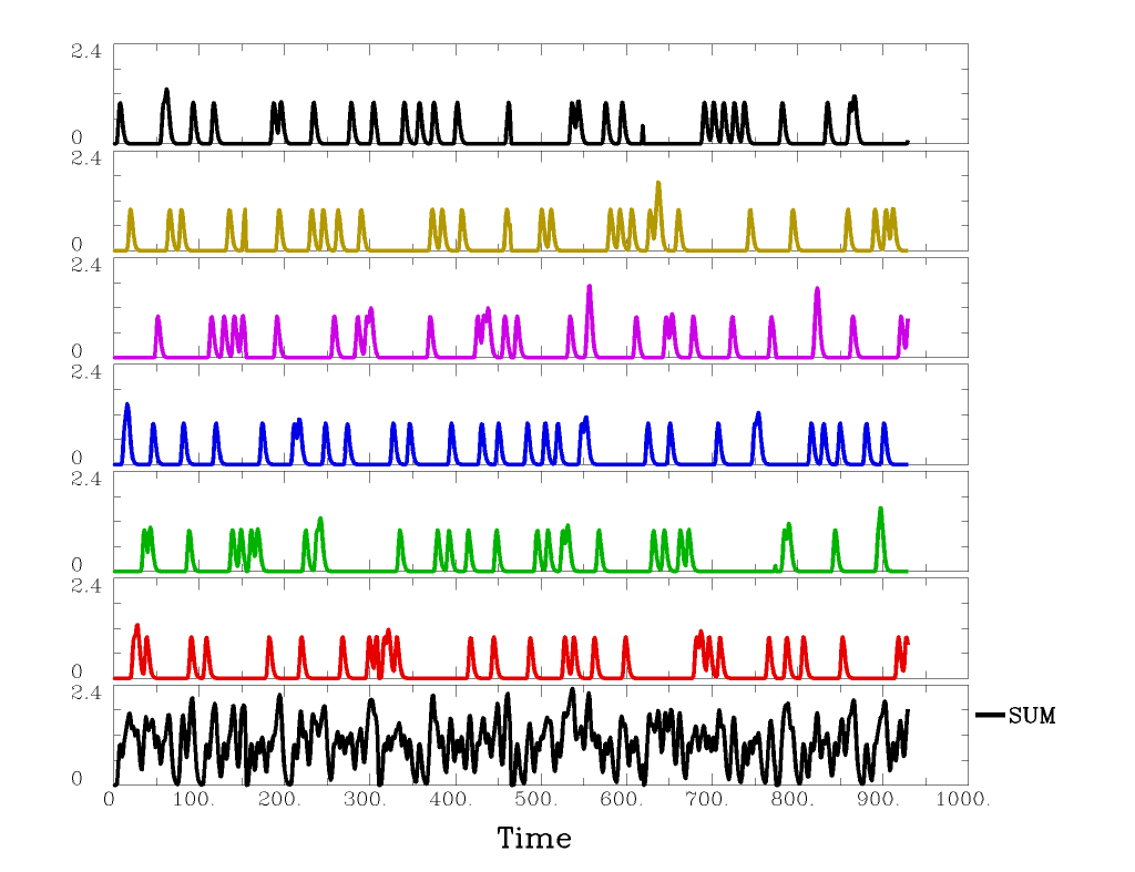
3dDeconvolve \
 -nodata 930 1.000 \
 -polort 2 \
 -concat '1D: 0 155 310 465 620 775' \
 -num_stimts 6 \
 -stim_times 1 bil-afni_cond_01.1D 'BLOCK(2,1)' \
 -stim_times 2 bil-afni_cond_02.1D 'BLOCK(2,1)' \
 -stim_times 3 bil-afni_cond_03.1D 'BLOCK(2,1)' \
 -stim_times 4 bil-afni_cond_04.1D 'BLOCK(2,1)' \
 -stim_times 5 bil-afni_cond_05.1D 'BLOCK(2,1)' \
 -stim_times 6 bil-afni_cond_06.1D 'BLOCK(2,1)' \
 -x1D X.xmat.1D -xjpeg disp.jpg

# compute the sum of non-baseline regressors
3dTstat -sum -prefix sum_ideal.1D X.xmat.1D'[18..$]'

# consider plotting the SUM below non-polort regressors
# command: 1dplot -xlabel Time -ynames SUM - sum_ideal.1D X.xmat.1D'[18..$]'
At this point, you can run the file myDeconvolve.txt (ex: sh myDeconvolve.txt > myoutput.txt), which will fit the matrices via 3dDeconvolve and estimate the ideal sum ideal waveform. If you choose to plot this, it will look something like:
To now get the relevant values, you now need to look in myoutput.txt. You can use awk, python or any other number of tools to extract these values, sum them, and then save that value as the “value to beat” for successive iterations. The goal is to find the smallest sum value of all of your different conditions. Essentially you are searching for the simulated design that will result in a design matrix with the smallest amount of unexplained variance.
Stimulus: Stim#1
 h[ 0] norm. std. dev. = 0.1182
Stimulus: Stim#2
 h[ 0] norm. std. dev. = 0.1148
Stimulus: Stim#3
 h[ 0] norm. std. dev. = 0.1163
Stimulus: Stim#4
 h[ 0] norm. std. dev. = 0.1135
Stimulus: Stim#5
 h[ 0] norm. std. dev. = 0.1202
Stimulus: Stim#6
 h[ 0] norm. std. dev. = 0.1193
Take that process and loop it a few thousand times and keep the design with the smallest std. deviation. Also worth noting, I didn’t show here that you can also add GLT (contrasts) to your model design and measure the standard deviation for those, which is also informative (sometimes more informative) to picking an ideal design. If you are looking for guidance, I just discovered that the AFNI group has an updated script that you can modify for your purposes.
In addition to modeling the efficiency for the evoked responses, you can add GLTs (contrasts) to your 3dDeconvolve command generated before to model the efficiency of the contrasts. This can be particularly useful if you have several stimulus classes going into one contrast of interest. The same process applies there, take the efficiency value and use that as the score to beat as you repeat the process in permutations.
Optseq2: Optseq2 provides similar functionality, albeit with slightly different options. The decision is yours, and often it is helpful to consider measuring the efficiency from optseq2 in AFNI via 3dDeconvolve. If you’re determined to use optseq, you can checkout the usage examples here.