While the information in this post is useful, I recommend users use TORTOISE for processing diffusion data.  You can read a tutorial of TORTOISE3 here.  

I previously described how to do some DTI analyses in AFNI.  To review, we could use a linear alignment to the b0 image in order to correct for some eddy current distortions.  There is also the option of aligning the data to the individual subject’s high-resolution anatomical data.  Whenever you do a motion correction, it’s recommended that you rotate your bvecs.  Following this, we fit the tensors using 3dDWItoDT, which in addition to linear fit (the FSL way), also offers a nonlinear tensor fitting algorithm.  Following the steps in the last post, you would end up with an individual subjects DTI data aligned to their anatomical data.  The next step is usually to do some type of tractography at the single-subject level.  AFNI now includes several tools for doing both deterministic tractography (3dTrackID) and probabilistic tractography (3dDWUncert & 3dProbTrackID).

So far we’ve performed the following steps on our data:

#make sure anatomical is in LPI orientation for generating GIFTI surfaces
3dresample -orient LPI -input Sag3D.nii.gz -prefix anat

#skullstrip output both an AFNI volume dataset (anat_ns+orig.HEAD) and a GIFTI anat_ns.gii)
3dSkullStrip -input anat+orig. -prefix anat_ns -o_gii anat_ns

#align the dwi data to the skull stripped anatomical
align_epi_anat.py -anat anat_ns+orig. -epi dwi+orig. \
-epi_base 0 -suffix _al2anat -epi2anat \
-anat_has_skull no -giant_move -tshift off \
-volreg_method 3dAllineate -epi_strip 3dAutomask -cost mi

#optional, but recommended, rotate b-vecs via see this post.
@rotatevectorsallx1 volreg_dset bvec.1D
#now fit tensors
3dDWItoDT -prefix DTI -automask -eigs -nonlinear -reweight -sep_dsets bvec.1D dwi_al2anat+orig.

At this point you need a couple of ROIs to find tensors between.  You can generate the masks by hand or by atlas, see this tutorial for ways to make ROIs and this one for helpful tips on combining them.  In this example I’ve created a couple of ROIs, combined them into the same mask via 3dcalc and resampled to the lower resolution via 3dresample (3dfractionize would also work).  To now perform the deterministic tractography, I use 3dTrackID, which implements the FACT algorithm with the added benefit of including the diagonals.  The program takes two masks as arguments, here I use the same file with different indices as my left and right ROIs.  I input the DTI files, give the program a text file of parameters and use the logic AND meaning the tracts found will involve BOTH of the ROIs.

3dTrackID -mode DET -netrois ROI_small+orig. \
-prefix o.TRACK_rois -dti_in DTI -algopt ALGOPTS_DET.dat -logic AND

The -algopt file has 8 values: 1) Min FA value; 2) Max Angle; 3) Min Length; 4) Number of Seeds in X; 5) Number of Seeds in Y; 6) Number of Seeds in Z; 7) Number of gradients (not currently used); 8) bvalue (not currently used).  The output will be a series of files beginning with o.TRACK_rois, including a MAP, a MASK, a Tract file, a stats file, and a trk (Trackvis compatible) file.  If we now wish to visualize the findings, we can use SUMA:

suma -npb 10 -i anat_ns.gii -niml &
DriveSuma -npb 10 -com viewer_cont -load_do o.TRACK_rois.niml.tract

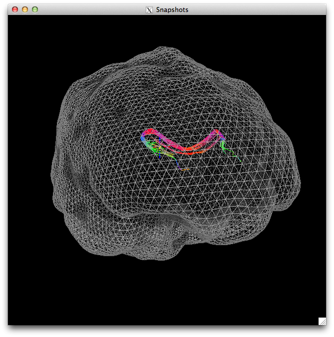
This code will generate a nice visualization, like the one below.  In SUMA, you can use the P key to change the density of the mesh being displayed.  The image below is one less than the original density.  You can then use the standard SUMA actions to view the identified tracts in whatever directions you wish.

Next time I will cover doing probabilistic tractography using the FATCAT programs 3dDWUncert and 3dProbTrackID.