Analyzing DTI Data in AFNI (Part 2)

While the information in this post is useful, I recommend users use TORTOISE for processing diffusion data.  You can read a tutorial of TORTOISE3 here.  

I previously described how to do some DTI analyses in AFNI.  To review, we could use a linear alignment to the b0 image in order to correct for some eddy current distortions.  There is also the option of aligning the data to the individual subject’s high-resolution anatomical data.  Whenever you do a motion correction, it’s recommended that you rotate your bvecs.  Following this, we fit the tensors using 3dDWItoDT, which in addition to linear fit (the FSL way), also offers a nonlinear tensor fitting algorithm.  Following the steps in the last post, you would end up with an individual subjects DTI data aligned to their anatomical data.  The next step is usually to do some type of tractography at the single-subject level.  AFNI now includes several tools for doing both deterministic tractography (3dTrackID) and probabilistic tractography (3dDWUncert3dProbTrackID).

So far we’ve performed the following steps on our data:

#make sure anatomical is in LPI orientation for generating GIFTI surfaces
3dresample -orient LPI -input Sag3D.nii.gz -prefix anat

#skullstrip output both an AFNI volume dataset (anat_ns+orig.HEAD) and a GIFTI anat_ns.gii)
3dSkullStrip -input anat+orig. -prefix anat_ns -o_gii anat_ns

#align the dwi data to the skull stripped anatomical
align_epi_anat.py -anat anat_ns+orig. -epi dwi+orig. \
-epi_base 0 -suffix _al2anat -epi2anat \
-anat_has_skull no -giant_move -tshift off \
-volreg_method 3dAllineate -epi_strip 3dAutomask -cost mi

#optional, but recommended, rotate b-vecs via see this post.
@rotatevectorsallx1 volreg_dset bvec.1D
#now fit tensors
3dDWItoDT -prefix DTI -automask -eigs -nonlinear -reweight -sep_dsets bvec.1D dwi_al2anat+orig.

At this point you need a couple of ROIs to find tensors between.  You can generate the masks by hand or by atlas, see this tutorial for ways to make ROIs and this one for helpful tips on combining them.  In this example I’ve created a couple of ROIs, combined them into the same mask via 3dcalc and resampled to the lower resolution via 3dresample (3dfractionize would also work).  To now perform the deterministic tractography, I use 3dTrackID, which implements the FACT algorithm with the added benefit of including the diagonals.  The program takes two masks as arguments, here I use the same file with different indices as my left and right ROIs.  I input the DTI files, give the program a text file of parameters and use the logic AND meaning the tracts found will involve BOTH of the ROIs.

3dTrackID -mode DET -netrois ROI_small+orig. \
-prefix o.TRACK_rois -dti_in DTI -algopt ALGOPTS_DET.dat -logic AND

The -algopt file has 8 values: 1) Min FA value; 2) Max Angle; 3) Min Length; 4) Number of Seeds in X; 5) Number of Seeds in Y; 6) Number of Seeds in Z; 7) Number of gradients (not currently used); 8) bvalue (not currently used).  The output will be a series of files beginning with o.TRACK_rois, including a MAP, a MASK, a Tract file, a stats file, and a trk (Trackvis compatible) file.  If we now wish to visualize the findings, we can use SUMA:

suma -npb 10 -i anat_ns.gii -niml &
DriveSuma -npb 10 -com viewer_cont -load_do o.TRACK_rois.niml.tract

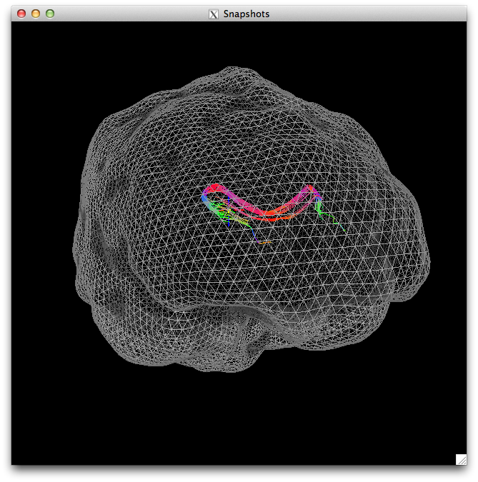
This code will generate a nice visualization, like the one below.  In SUMA, you can use the P key to change the density of the mesh being displayed.  The image below is one less than the original density.  You can then use the standard SUMA actions to view the identified tracts in whatever directions you wish.

Suma_vis2

Next time I will cover doing probabilistic tractography using the FATCAT programs 3dDWUncert and 3dProbTrackID.

Writing your own fMRI programs using the AFNI API (Part 1)

I find that it’s fairly rare that I wish there was an AFNI program that did something that cannot be accomplished with existing tools and a bit of creativity.  But, if you do find something that requires writing a custom program, the AFNI distribution is both easily accessible and fairly straightforward to code for.  Over the next several months, I will cover how to program some very basic programs via the AFNI API (API = Application Programming Interface).  I primarily target Mac users here because 1) I’m writing this on a Mac; 2) writing instructions for every breed of Linux is exhausting.

To start, you will need to get the AFNI Source code (link).  Download and unpack the source into a directory that you will use for all of your AFNI development purposes.  Now it’s important to note that you don’t need to build the entire distribution in order to write your own programs.  Some of the harder to compile components of AFNI are responsible for drawing the GUI to the screen.  Skipping these makes our life easier, and usually AFNI programs run from the command line anyway.  With this in mind, the next step is to make a copy of the Makefile that best describes your Mac OS version (mine is Makefile.macosx_10.7_Intel_64) inside the source distribution.  Rename the copy simply “Makefile”.

If you have installed AFNI with Fink to satisfy the dependencies, you may already have what you need.  But as many of you know from previous posts, I suggest that you don’t use fink and instead use Homebrew.  First install Xcode and then via the Xcode Menu –> Preferences –> Downloads, install the Command Line Tools.  Now you can install homebrew, and then will need to install a few packages to aid in compiling.

brew install libpng jpeg expat freetype fontconfig

If you are using Homebrew, open the Makefile that you created and change any place where it says /sw to /usr/local.  Also, if you don’t want to install gcc via homebrew, change all of the references to GCC to be /usr/bin/gcc instead of the default /usr/local/bin/gcc.  Once these changes have been made, save and close your Makefile.

For both Homebrew and fink users.  Open a terminal window, and navigate to the AFNI sources folder.  To make your own AFNI programs, you mostly just need to build libmri.a, to do this just execute the following in your shell:

make libmri.a

Wait a while for the compiling to complete.  You should then see a file created called libmri.a.  This file (a library, or framework depending on your terminology) allows you to access any file type that the AFNI distribution supports (e.g. AFNI HEAD/BRIK and NIFTI and NIFTI Compressed).  At this point you can try to build a sample program to make sure everything is working.  The simpler programs can be found via

  cd afni_src
  wc 3d*.c | sort -n | head

In this case, I’ll use 3dEntropy as an example.  I’m not modifying the program at all for this, just changing the output name to 3dTest.  Notice the -I is telling GCC where to find all of the include headers and -L is telling the compiler where to find any linked libraries (e.g. libmri.a).  To test compile a program, try the following from inside of your AFNI source directory:

gcc 3dEntropy.c -o 3dTest -lmri -lXt -lf2c -lz -lexpat -I nifti/niftilib/ -I nifti/nifticdf -I nifti/znzlib -I /opt/X11/include/ -I rickr -L . -L /opt/X11/lib/

There you have it.  Test your program to see that it generates a help file and away you can go with writing your own AFNI programs.  I’d like to thank Daniel Glen and Rick Reynolds of the AFNI team for helping me get this setup working on my own computer.  I hope that by posting these instructions, others won’t have to ask as many questions as I did!

Happy coding!

Fun with AFNI Masks

I watched an episode of The Big Bang Theory last night where Dr. Sheldon Cooper was airing an episode of “Fun with Flags,” which gave me the idea for today’s blog post title.  A while ago, I detailed how to create ROIs in AFNI using a variety of different methods.  And I even included a quick bit about combining multiple masks into a single file.

To start off, last time we used an Atlas to create masks for the Middle Frontal Gyrus (MFG).  To generate these for each hemisphere we use the following two commands:

whereami -mask_atlas_region CA_N27_ML:left:middle_frontal_gyrus -prefix l_mfg
whereami -mask_atlas_region CA_N27_ML:right:middle_frontal_gyrus -prefix r_mfg

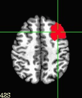
To illustrate, the first command would generate only the mask below:

left_only


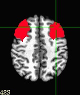
If we then wanted to combine the left and right hemisphere masks, we could use 3dcalc (associated mask shown below command):

3dcalc -a l_mfg+tlrc. -b r_mfg+tlrc. -expr 'a+b' prefix l+r_mfg

l+r


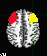
Now this mask can be used with any of the AFNI tools (e.g. 3dmaskave, 3dmaskdump, 3dROIstats to name a few).  But the problem here is that both ROIs have the SAME value, meaning that any ROI tool isn’t going to easily differentiate the left and right MFG.  This may be what you want, but you might also want to look at these ROIs separately.  To do this, we use a slightly different 3dcalc command (output shown below):

3dcalc -a l_mfg+tlrc. -b r_mfg+tlrc. -expr 'a+2*b' -prefix l+r_mfg_sep

l+r_sep

This “combined yet separate” mask will allow us to use 3dmaskave or 3dROIstats to output different values for each hemisphere!  The easy approach is to use 3dROIstats:

3dROIstats -mask l+r_mfg_sep <dataset1> <dataset2> ... <dataset n>

You can also ask 3dmaskave or 3dROIstats for only the mask of a particular value using <n> where n is the value of the mask of interest.  For example:

3dmaskave -mask l+r_mfg_sep+tlrc.'<1>' mydataset+tlrc.HEAD
3dROIstats -mask l+r_mfg_sep+tlrc.'<1>' mydataset+tlrc.HEAD

Both of these commands will output the data for only the LEFT MFG!   I’ll wrap up with a somewhat more complex example.  Imagine that you used Freesurfer to create ROIs for each individual subject’s MFG.  If you wanted to compute a group mask for the MFG, you could then warp each subject’s MFG ROI to standard space (@auto_tlrc) and then use 3dmask_tool to create a mask where at least 50% of your subjects have a mask present.

3dmask_tool -input mfg_mask_subject???+tlrc.HEAD -prefix overall_mask -frac 0.5

you can adjust the -frac to adjust the percentage of masks that need to overlap that area before a final mask is made.  You can also use -union to get the overall mask across all subjects (similar to doing a 3dMean, followed by 3dcalc -expr ‘step(a)’).  3dmask_tool also has also allows you to fill holes in masks, combine them, dilate and erode the masks, etc.

Multiple Basis Functions with afni_proc.py

Admittedly the title is a little bit opaque, you can already use afni_proc.py to have some of your regressors use the GAM basis function and others to use another basis function (e.g. SPM).  But one thing that I find helpful is to compare a standard basis function (e.g. GAM, SPM, SPMG2, etc) with an FIR style basis function (e.g. TENT).

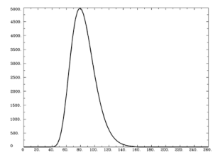
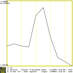
One major reason to advocate an FIR/TENT model is that you make no assumptions of the shape of the HRF.  The downside to this is that you “burn” degrees of freedom in your model in order to estimate the shape at each time point.  Whereas GAM and similar basis functions have a standard shape that uses fewer degrees of freedom to estimate.  For reference, GAM and TENT models are shown below.

Gamma

TENT


But this post isn’t really about the differences between the models.  Instead, we want to be able to run GAM first and then TENT on the same data without going through the entire reprocessing pipeline that afni_proc.py suggests as the defaults.  There is good news, you can do this without too much trouble, you just have to know where to get the correct files!

With that, let’s jump in.  My file structure of choice works like this:

SubjectFolder
-- anat/high_res.nii.gz
-- func/epi runs
-- stim_times/timing text files
-- SubjectFolder.GAM

So within any given subject folder, I have all of the necessary input files for afni_proc.py, in addition to the output folder from the first pass analysis using afni_proc.py inside SubjectFolder.GAM.  Inside this output folder are all of the necessary files to go straight into my regression step of a new afni_proc.py script.

At this point I just need to write a new afni_proc.py script that copies the motion parameters from the previous volreg, the high resolution anatomical data,  the stimulus timing files, and of course the full preprocessed datafiles (pb.03 in this case).  I’ve included a script below:

afni_proc.py -subj_id $aSub -script afni_$aSub_fastlocTENT.tcsh -out_dir $aSub.TENT \
 -dsets $aSub.GAM/*pb03*.HEAD \
 -blocks mask regress \
 -copy_files $aSub.GAM/*anat_final* \
 -regress_stim_times $aSub.GAM/stimuli/times* \
 -regress_stim_labels print speech \
 -regress_local_times \
 -regress_reml_exec \
 -regress_motion_file $aSub.GAM/dfile_rall.1D \
 -regress_basis 'TENT(0,12,7)' \
 -regress_censor_outliers 0.1 \
 -regress_censor_motion 0.3 \
 -regress_est_blur_epits \
 -regress_est_blur_errts \
 -regress_opts_3dD \
 -num_glt 11 \
 -gltsym 'SYM: +print' -glt_label 1 'print' \
 -gltsym 'SYM: +speech' -glt_label 2 'speech' \
 -jobs 8 \
 -bash -execute

One other thing to note about this afni_proc.py script, it uses the TENT basis function and then use the GLTs to give the overall average area under the curve for the entire 12 second basis function.  Note that my TR is 2 in this experiment, which is why there are 7 “TENTs” to fit.  As an alternative, I could have also used TENTzero, which would force the first and last values of the basis function to be zero.  I’ve found this approach to be very helpful.

Analyzing ERP Data with PCA-ANOVA in R

Running a PCA-ANOVA in R is fairly straightforward.  In this post we’ll focus on doing a temporal PCA on clusters of ERP channels.  First you will want to arrange the data in one file.  If you are coming from Net Station, you can export your ERP averaged files to text and then use MCAT to create averaged channels to input into the PCA.  MCAT does three things that are useful in this case: 1) MCAT creates average channels; 2) MCAT rotates the channels so that the columns represent time, instead of the EGI default method of columns representing different channels; 3) MCAT will concatenate all of the subjects together.

By default, MCAT creates 10 channels from a 128 channel EGI Net.  It is simple to modify the number and composition of each channel, but for the purposes of this walkthrough, we will use the defaults.  The default are 5 channels per hemisphere, representing Frontal, Central, Temporal, Parietal, and Occipital regions.  In this example, we have 24 subjects and they see two conditions: congruent and incongruent.

In order to run a PCA with rotation in R, we will need the psych package:

install.packages('psych', depend=T)

Next we want to read the data into R

thedata = read.table("demo_500.txt", sep='\t', header=F, skip=0)

This will read the text file into R, noticing that it is tab-delimited and has no “header” which would be a listing of variables.  If you used MCAT, you are likely going to use this line as is.  The next step is running the PCA in R.  To do so, we use the following command:

my.pca = principal(thedata[seq(26,150,2)], nfactors=5, rotate='varimax', scores=TRUE, covar=F)

Stepping through this command, this will run a PCA on time points 26-150, skipping every other time point.  I chose these values because my ERP included 100 millisecond baseline, recorded at 250Hz, breaks down to 4 milliseconds per sample, 25*4=100.  We don’t want to include the baseline in the PCA for this example.  I skip every other sample because of the high temporal correlation in the data and skipping every other value will give you plenty of resolution to detect the “slow” ERP components.  You should feel free to try it both ways.  Next, we are going to start with 5 components and use a varimax rotation, which will force the components to be orthogonal.  Finally, this is running the PCA using a correlation matrix, the alternative is to use a covariance matrix.  The result is that a correlation matrix will add a bit of normalization to your PCA.

Truthfully, I had some difficulty getting the covariance matrix PCA to give me the same values as other software packages (e.g. SAS).  The Correlation Matrix results were almost identical to SAS.  I’ll debug this later.  

At this point, we need to see if 5 components correctly captures the variance of the original data.  To do this, most people use the Scree plot, originally developed by Cattell.  The general idea is to retain the factors until you reach the point where the rocks would collect at the base of a mountain.  Alternative solutions to choosing the number of factors are 1) retain values until you reach an Eigan Value of 1.0; 2) retain values until you account for a pre-determined percent of the variance.  Both of these methods will unfortunately leave you with factors that account for very little variance.  The validity of using these low-variance components for later analyses is arguable, though I tend to avoid using them.  You can see in the scree chart below that we would choose between 5 and 6 components.  For the sake of ease, today I will choose 5.
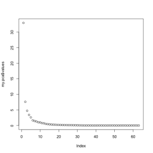
scree

At this point, the PCA has created 5 factors that represent each CHANNEL (or averaged channel) for each condition, for each subject.  Going into the PCA you had 2 conditions, 10 channels, and 24 subjects, which was represented as 480 rows in the input file.  Now for each of those 480 rows, you have 5 values, representing the data reduced time course of each channel within condition within subject.  The next step is to rename these factors to represent the appropriate channel and conditions as well as organize them into one row for each participant so that you can do repeated-measures ANOVAs on the data.

The following code rotates the matrix, to make renaming easier.  Then we cast the data frame as a matrix and re-specify it to be 24 rows (the number of subjects).  Then we send it back to a data frame and add “labels” to the data frame representing each channel, condition, and factor.  Channels are here labeled as the first two letters, so FL would be “front left” and so on.

rotdata = t(my.pca$scores) #rotates the data.frame
rename = matrix(rotdata, nrow=24, byrow=TRUE) #nrow = #subjects
rename = data.frame(rename); #convert it back to a dataframe
labels = c("FLcon1 FLcon2 FLcon3 FLcon4 FLcon5 FRcon1 FRcon2 FRcon3 FRcon4 FRcon5 CLcon1 CLcon2 CLcon3 CLcon4 CLcon5 CRcon1 CRcon2 CRcon3 CRcon4 CRcon5 PLcon1 PLcon2 PLcon3 PLcon4 PLcon5 PRcon1 PRcon2 PRcon3 PRcon4 PRcon5 OLcon1 OLcon2 OLcon3 OLcon4 OLcon5 ORcon1 ORcon2 ORcon3 ORcon4 ORcon5 TLcon1 TLcon2 TLcon3 TLcon4 TLcon5 TRcon1 TRcon2 TRcon3 TRcon4 TRcon5 FLinc1 FLinc2 FLinc3 FLinc4 FLinc5 FRinc1 FRinc2 FRinc3 FRinc4 FRinc5 CLinc1 CLinc2 CLinc3 CLinc4 CLinc5 CRinc1 CRinc2 CRinc3 CRinc4 CRinc5 PLinc1 PLinc2 PLinc3 PLinc4 PLinc5 PRinc1 PRinc2 PRinc3 PRinc4 PRinc5 OLinc1 OLinc2 OLinc3 OLinc4 OLinc5 ORinc1 ORinc2 ORinc3 ORinc4 ORinc5 TLinc1 TLinc2 TLinc3 TLinc4 TLinc5 TRinc1 TRinc2 TRinc3 TRinc4 TRinc5"); #assign variable names
names(rename) = unlist(strsplit(labels, split=" ")); #put names into dataframe

I make these labels in the SPSS Label Maker and so I have R split the continuous string of values into separate values. At this point you have a data frame “rename” that has 24 rows and 100 variables (10 electrodes * 2 conditions * 5 factors = 100 variables).  At this point you are ready to run an ANOVA on each of the five components that were extracted.  I like how easy this is to do in the “ez” package, so we’ll outline those steps:

factor1 = names(rename[seq(1,100,5)])
f1 = rename[factor1]
f1$subject = seq(1,24)

These three lines breakout the first factor into a second dataset.  We then use melt() to convert the data from wide format to long format.  Next we need to add some descriptors to the data, these are variables in long format that serve to describe characteristics of that particular data point.  I use rep to do this and exploit the organized format of the data.  Using the code below, I add variables region, hemisphere, and condition.  You could also do this with a series of functions of if/then or ifelse() commands.

longdata = melt(f1, id.vars=c("subject") )
longdata$region = rep(c('F', 'C', 'P', 'O', 'T'), each=48) #2 hemispheres, 5 regions, 24 subjects
longdata$hemisphere = rep(c('L', 'R'), each=24)
longdata$condition = rep(c('con', 'inc'), each=240)

Finally we are ready to actually run the ANOVA on this first factor with a condition X hemisphere X region repeated-measures design.

library(ez)
ezANOVA(longdata, dv='value', wid=subject, within=.('condition', 'hemisphere', 'region'), type=)

The results are nicely printed out, a subset is shown below.  We have identified a main effect for hemisphere as well as region, these are qualified by a hemisphere X region interaction.

$ANOVA
 Effect DFn DFd F p p<.05
2 condition 1 23 0.06986913 7.938816e-01 
3 hemisphere 1 23 7.88955879 9.965560e-03 *
4 region 4 92 9.88646606 1.066086e-06 *
5 condition:hemisphere 1 23 0.11050484 7.425808e-01 
6 condition:region 4 92 1.04554033 3.881822e-01 
7 hemisphere:region 4 92 3.91039384 5.607436e-03 *
8 condition:hemisphere:region 4 92 1.24818805 2.962026e-01

Now that you’ve identified main effects or interactions in this first factor, you can repeat the process for the other factors.  Finally you can see where the factors were most active by looking at the “factor loadings” These are exposed in R and the Psych toolbox as by running:

my.pca$loadings

Most people seem to agree that a loading of 0.4 or higher (absolute value) are worth reporting.  Next EEG post, I’ll show how to do the same analyses using the ERP PCA Toolkit that was talked about before.