To Eric Langlois

Eric

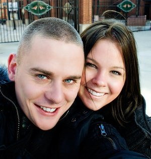
On a personal note, I would like to say a few things about my friend Eric Langlois.  Eric recently passed away.  Several others (here, here, here) have posted about his unfortunate death, and the story can be found here.  Eric was a Connecticut-based photographer and founder, owner, and principal photographer for Raw Photo Design.   He was an amazing photographer (see his Raw Photo Design blog), helping to capture the happiest moments of people’s weddings, engagements, and everyday meeting up with friends like me at one of the many New Haven, Connecticut pizzerias.  I wanted to write some of my memories, both for myself and hopefully for those of you lucky enough to know him or know of him.

Before Eric started his own photography business, he worked at the Yale Child Study Center (CSC) as a Research Associate.  I first met Eric in 2006 when I was an intern at the CSC.  I had just graduated from my Master’s program in Louisville, Kentucky and was moving to New Haven to get some lab experience before applying to graduate schools.  Having never been to Connecticut, I needed a guide and Eric volunteered to show me around and even help me find housing!  Without knowing me, Eric scouted several different apartments so he could recommend the best places to live.  When I arrived at Yale, Eric helped me get a bed, some Ikea furniture and the the infamous Ikea meatballs (as well as $0.50 hot dogs and cinnamon rolls).  He also introduced me to the New Haven Food Trucks, and proceeded to make fun of me for eating Chinese food several days in a row.

I only stayed at Yale for 6 months before getting into graduate school at the University of Houston in Texas, but in 2007 I returned for the summer as Eric was transitioning from a full-time Yale employee to a part-time photographer.  When I returned in 2009, Eric’s photography business had taken off.  Despite his flourishing business, Eric made the hour drive to New Haven to visit me on my first day back at the CSC.  He showed me what he was working on and we went to dinner (pizza of course).  We caught up and he offered to teach me how to take better photos.  Over the next several years, Eric would give me a call whenever he was coming to town so we could meet up for food and talk science, photography, and Ikea.  Inevitably, he would get a parking ticket every time, but he still would text me later to say how glad he was that we got to hang out, even if only for a hamburger at Louis Lunch or a walking lunch across town as he was headed to meet a new client.  Eric exemplified the friend who was always there, even though you don’t see them on a regular basis.  He would send emails in the middle of the night to touch base while editing photos for a new project that reminded him of an obscure memory involving the two of us.

To my friend Eric, I wish we had more time and I wish that we had talked more.  I will always remember you.  And each time I pick up a camera or go to Ikea, I will continue to smile to myself as I remember how you approached life with such joy and happiness that always made the people around you just as happy.  I always imagined that you would be the photographer for my eventual wedding and the extra care and detail you always took when post-processing each and every photo.  In 2009, I attended 13 weddings, and I never found a photographer who had the ability to connect instantly with people at a wedding.  You managed to capture so much more than the ceremony, the clothes, and the dancing.  I hope that your new adventure is amazing…

Please consider donating to the Eric Langlois Family Fund to help his wife and children.

Installing the ERP PCA Toolkit

Today I’m raising awareness of a phenomenally helpful tool in ERP Research called the ERP PCA Toolkit.  In short, the PCA toolkit allows you perform temporal, spatial, and complex (e.g. temporo-spatial) analyses on ERP data.  Shown in the figure below is a quick temporal-spatial PCA on some ERP data for a go/no-go task.  The PCA pulled out a temporal component that peaked at 774 milliseconds and a spatial component in the right parietal lobe (electrode 97 on an EGI Hydrocel Net).

If you’ve never used a PCA to help identify regions of temporal or spatial interest in your ERP data, I highly recommend using the PCA Toolkit.  I will post some R code in the future that will show how to do a PCA by hand, which helps explain the fundamental steps, but there is something to be said about the efficiency of using a Toolkit like this one to really see what your data has to offer.  It’s worth noting that while this is an ERP toolkit, I’ve had some luck using it on MEG data, though typically we use MEG to go straight to dipoles or activation in the brain (MSI).

PCA_Toolkit


One of the first hurdles of using any MATLAB toolbox is to get it installed correctly.  The PCA Toolkit uses routines from several different packages, including FieldTrip and EEGLAB.  You will want to get the most recent releases of both of these packages and the ERP PCA Toolkit before following the steps below to install the PCA Toolkit.  I usually put my MATLAB toolboxes in a Shared Folder, on Macs I prefer to use /Users/Shared/.

  1. Add PCA Toolkit to your path
    1. Add with Subfolders
  2. Add EEGLab to your path
    1. Add just the EEGLab folder, not the subfolders, EEGLab will take care of the rest of you!
    2. Remove the “slimmed down” FieldTrip install included in EEGLab by deleting the fileio and fieldtrip-partial directories in the “eeglab/external” folder
    3. Disable the “binary ICA” path by setting line 56 (or so) in eeglab/functions/sigprocfunc/icadefs.m to read ICABINARY = [];
  3. Add FieldTrip to your path
    1. Add just the folder.  Click Save, then type “ft_defaults” into the MATLAB console
    2. Go back to the Set Path dialogue and notice FieldTrip has added several things, click “Save”.

These instructions are direct from the “tutorial.pdf” file included in PCA Toolkit.  If you find the toolkit helpful, remember to 1) send an email to Dr. Joseph Dien and thank him for his excellent work and 2) cite the toolbox in your papers:

Dien, J. (2010). The ERP PCA Toolkit: An open source program for advanced statistical analysis of event-related potential data. Journal of Neuroscience Methods 187(1), 138-145.

Some examples of using PCA Toolkit coming in a later post.

Parallelizing Freesurfer

Today I started running VBM and Freesurfer comparisons on a “new” dataset that everyone in our lab is particularly interested in moving forward.  The VBM was all carried out in SPM8 with the VBM8 toolbox. I particularly like the VBM8 toolbox because it makes use of the SPM8 DARTEL transformations, and it’s relatively easy to queue up a lot of jobs and come back a day later to all of your data segmented (grey matter, white matter) and normalized to MNI space.

But I also wanted to process this data through Freesurfer.  So you have a few options, you could 1) Open a new terminal window for each and every brain that you wish to process, limited by the total number of processors (or RAM) on your computer, and wait for those to finish before starting a new batch of processing (this requires a lot of remembering to start the next batch); 2) you could use a for-loop script to automatically start the next brain, which would take you approximately 12-hours (I’m using 12 hours to make the math simple, sometimes it takes longer) multiplied by the total number of subjects (in this case 12 hours * 50 subjects = 25 days).

for aSubject in Subject*.nii.gz
do
    recon-all -s ${aSubject%.nii.gz} -i $aSubject -all -qcache
done

Or 3) you could use GNU Parallel to batch process all of the brains using a set number of processors and have it automatically start more processing as each individual subject finishes.  I have a chunky Mac Pro on my desk with 12-cores and 40GB of RAM, I estimate that I can run 12 simultaneous processes and still not run out of RAM (and since I have hyperthreading, I shouldn’t find my computer grinding to a halt).  Total processing time is roughly (12 hours * 50 brains)/12 processors = 50 hours or just over 2 days.  Considerably faster than doing one at a time or constantly checking in to start more processing.

If you want to install GNU Parallel on linux see this post; if you have a Mac, I highly recommend using homebrew (requires the FREE Apple Xcode), followed by a quick “brew install parallel”.  Once you have GNU Parallel installed, I’m going to use – ls – to get a list of all NIFTI files in a directory, pipe that through sed to remove the extension (.nii.gz) and then pipe that list of subjects to GNU Parallel to automatically queue up jobs with a maximum of 12 simultaneous processes.  Press enter to begin the process.

ls Subject*.nii.gz | sed 's/.nii.gz//' | parallel --jobs 12 recon-all -s {} -i {}.nii.gz -all -qcache

It’s really that easy, when each job finishes, it will spit out the output to the terminal.  Remember that Freesurfer also spits out individual log files for the recon-all process into each subject’s folder.  A quick look at top or Activity Manager will show that I have several processes of Freesurfer running simultaneously.  When these finish, more will automatically start.

p_freesurfer


If you want to be daring and have several computers running the same architecture, operating system, and version of Freesurfer, you can use GNU Parallel to use multiple computers, complete with copying the files over and transferring results back.  Alternatively, if you have shared storage (e.g. NFS Mounts), you can just issue the commands to all of the computers that way.

Visualizing Single Subject DTI Data (FSL)

A few posts ago, I described how to do some basic analyses of Diffusion data.  I realize now that I left off the visually cool factor of displaying individual subject data.  Once you complete the eddy_correct and dtifit steps in the previous post, several files will be generated for FA (fractional anisotropy), MD (mean diffusivity), Lx (eigenvalue #) and Vx (eigenvector #), among others.

The easiest way to visualize the single subject data is to use FSLView.  I prefer to launch FSLView with the files that I need to visualize included on the command line.

fslview dti_run1_FA.nii.gz dti_run1_V1.nii.gz

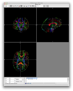
This will launch FSLView with both the FA and First Eigenvector .  Now at the bottom of the window, select the V1 image and click the purple I button for info.  Change the display as to RGB and the Modulation to your FA image.

info_FSL_DTI

And just like that, you should have some nice colormaps for your DTI data.

Screen Shot 2013-06-06 at 10.49.45 AM


You can of course change the views in FSLView to Lightbox or whatever other view you prefer.  We tend to make figures in Lightbox view for later review, just to keep track of all the data and to make sure nothing strange makes it through to the final group analysis.

Single Subject Analysis in AFNI

AFNI has three major avenues to running a single subject analysis.  1) You can use uber_subject.py to configure the analysis in a Graphical User Interface (GUI); 2) You can use afni_proc.py to specify the analysis using the command line; 3) You can write your own command line commands in your own script, which calls each AFNI program as needed with the settings that you desire.

The major problem with approach #3 is that AFNI has thousands of options across more than 100 programs!  This is part of the reason why AFNI had such a steep learning curve.  But fortunately, options #1 and #2 are considerably easier for both the new AFNI user and the experienced AFNI user alike.  In quick summary, uber_subject.py provides a GUI interface for setting up your analyses.  Underneath that GUI, uber_subject.py calls another python script called afni_proc.py.  Now here’s an important distinction – afni_proc.py has many many many more options than uber_subject.py for configuring your analyses.  But try as I might, for easily 75% of my analyses, uber_subject.py has all of the options you will need turned on by default.

And with that, let’s look at uber_subject.py!  The program itself comes installed with AFNI, but to get everything working requires the installation of PyQT.  If you want some guidance on that, checkout the previous post for Mac Installation instructions.  Typing “uber_subject.py -help_install” on any platform will give you the AFNI group’s recommendations for installing the necessary dependencies.  Launch uber_subject.py by typing its name into the terminal window on a Mac or Linux and be presented with the following:

Screen Shot 2013-05-29 at 9.44.45 AM


Notice the scrollbar on the right side indicating more options below!  In addition, clicking on checkboxes to add options may increase the length of the scrollbar.  Let’s fill in the options with some reasonable defaults (some people may find other defaults more reasonable than these).  These options will setup AFNI to perform outlier detection, slice timing correction, perform a single transformation aligning the EPI to the high resolution anatomical with motion correction and the warp to MNI space, spatial smoothing, masking, converting the scanner units into standard units (for % signal change), and running the regression via 3dDeconvolve with motion parameters entered in.

Subject ID: A subject ID or Name or identifier
Group ID: If you have multiple groups, use the name here, otherwise “all” or the name of the study works well
Analysis Initialization: This allows you to set analyses for either “task” or “resting” and let’s your specify analyses in the volume or on the surface.  For most analyses, I tend to start with a “task” and in the volume.  In part because the surface requires a good FreeSurfer or Caret cortical surface.  If you are new to AFNI, leave the processing blocks to the default.
Anatomical Dataset: This is your high resolution image (think MRPAGE or SPGR).
EPI datasets: These are your function EPIs.
Stimulus Timing Files: these are AFNI specific timing files.  They should be in text format with one file per stimulus condition and one line in each file per run.  So if you have two runs, you would have two lines in each stimulus file.  If you have a stimulus condition that only appears in one run but not the other, add a * to let AFNI know that it has a blank line.  After you add them to uber_subject.py, add a label by clicking on the empty label box and typing one in.
Symbolic GLTs: Are your “contrasts”, here you can specify the difference between Condition A and Condition B or any other combination that you wish.  If this seems daunting, click the “init with examples” to see some generic contrasts that relate to your stimulus labels.
Expected Options: These are a series of useful options.  First TRs to remove include your pre-steady state images, but only if your stimulus timing files reflect the removal of these.  Volume register base options are first, third, and last.  Since I trim off the first several TRs on my imags, I tend to use first.  Blur size is important, start with two voxels (in my case this is 4mm) if you’re new and then google blur size impact on fMRI.  If you’re an old hat, fill in your value here.  Motion censor, I would stick with the defaults.
Extra Regress Options: Change the outlier censor to 0.1 (censors a TR if 10% of voxels are outliers).  Jobs can be set to the number of processors on your computer.  Even if you have 24 cores, I wouldn’t really set this higher  than 12.  GOFORIT should stick with the defaults.  bandpass is usually left blank.  I also add the 3dREMLfit option.
Extra Align Options: I use the default LPC, but add “use giant_move” as the high resolution image is typically in a very difference space than the EPI.
Extra tlrc options: These are additional options for the warp to standard space.  I use the defaults of TT_N27+tlrc and the option to strip the skull.  You can view the different templates and make your own decision there.

Now that you’ve specified all of the options, click the button in the upper left that looks like a text document in a rectangle.  This will show two text windows, the first shows you the script that will be run, notice that it calls afni_proc.py.  The second shows the variables that uber_subject.py used to construct the script.  Importantly, you can modify this generated script if you want to add or change options.  Just remember to save with command or control + S.  To run the script press the green circle button in the upper left of the uber_subject.py window.  A progress window will show up to show you your analyses being run.

Now that you’ve run one subject, repeat the process for all of your other subjects.  Alternatively, copy the afni_proc.py script generated by uber_subject.py and modify it for each subject.  After you’ve run all of your subjects, you can do group analyses with a number of tools to be described later – including uber_ttest.py.