I receive a lot of questions about how to setup the basic analyses in AFNI. Previously I detailed using uber_subject.py, the AFNI graphical user interface to afni_proc.py which really does all of the hard work under the hood. Today I’m going to briefly review the common options in afni_proc.py and why I use them. You can use the script generated from uber_subject.py as a nice starting point or Example 6 from the afni_proc.py help.
So let’s start off with my file structure. Often when I convert files from DICOM to NIFTI, all of the NIFTI files end up in one directory. I like to organize them around what their purpose is so that when I write scripts, things get easier. So first of all, I put all of the anatomical images into a folder called “anat” and each experiment has several EPI files that each go into a folder called func_something, where the something is an easy way of describing what the experiment is. In this case, I’m processing data from a fast localizer, which has two conditions, one for print and one for speech. The third necessary folder is a stim_times folder, this is where I keep all of my stimulus timing files. in this case, I only have two conditions, but in other experiments where I have 9 conditions, things can get cluttered very quickly. That said, one particular subject might look like this:
Subject001
--anat
----Sag3dMPRAGE.nii.gz
--func_fastloc
----ep2dbold_001.nii.gz
----ep2dbold_002.nii.gz
--stim_times
----condition_01.txt
----condition_02.txt
Once I have my folders organized in this manner, I can run the following script within each folder (or loop through using a shell script). This will tell afni_proc.py where the functional and structural images are. More breakdown of what each step does below.
afni_proc.py -subj_id ${aSub} \
-script afni_fastloc_${aSub}.tcsh \
-out_dir ${aSub}.fastloc \
-dsets func_fastloc/*ep2dbold*.nii.gz \
-blocks tshift align tlrc volreg blur mask scale regress \
-copy_anat anat/*Sag3D*.nii.gz \
-anat_has_skull yes \
-tcat_remove_first_trs 6 \
-tshift_opts_ts -tpattern alt+z2 \
-tlrc_opts_at -init_xform AUTO_CENTER \
-align_opts_aea -giant_move \
-volreg_align_e2a \
-volreg_align_to first \
-volreg_tlrc_warp \
-blur_size 8 \
-regress_stim_times stim_times/condition_??.txt \
-regress_stim_labels c1 c2 \
-regress_local_times \
-regress_basis 'GAM' \
-regress_reml_exec \
-regress_est_blur_epits \
-regress_est_blur_errts \
-regress_censor_outliers 0.1 \
-regress_censor_motion 0.3 \
-regress_opts_3dD \
-num_glt 3 \
-gltsym 'SYM: +c1' -glt_label 1 'print' \
-gltsym 'SYM: +c2' -glt_label 2 'speech' \
-gltsym 'SYM: +c1 -c2' -glt_label 3 'print-speech' \
-jobs 8 \
-bash -execute
So what does it all mean, that’s the question that comes up fairly often. I find it helpful to go a few lines at a time in understanding what you’re asking afni_proc.py to do. Also, after you run the script, you will see that afni_proc.py simply generates a LONG tcsh file that runs the analyses on each subject. You can always view what this script is doing as well.
The first three lines (shown below), tell afni_proc.py the subject name (useful for naming files), the name of the script to create (useful if you want to run multiple iterations of the script), and the output directory to save all of the data to (also useful if you run the script with different permutations).
afni_proc.py -subj_id ${aSub} \
-script afni_fastloc_${aSub}.tcsh \
-out_dir ${aSub}.fastloc \
Next we tell afni_proc.py which “blocks” of analysis code we wish to run. You can always change or reorder these if you wish. Here we are asking the script to perform sinc interpolation (a.k.a. time shifting, slice timing correction), next it will align the EPI and anatomical images (co-registration), create a normalized image in standard space (you can select which template to use!), perform motion correction (realignment), apply a spatial smoothing kernel, create a mask (but not actually apply it in single-subject analysis unless you tell it to), and run the regressions using 3dDeconvolve. One thing to note, some people will wonder why we place the co-registration and normalization before realignment/motion correction. It’s because AFNI will actually take all three of these spatial transforms and concatenate them into a single transform. This is useful in that it only has to perform interpolation once on your data.
-blocks tshift align tlrc volreg blur mask regress \
The next three lines tell us about our data, here we tell the script where the anatomical data is, that it has a skull (or that it doesn’t), and that in the functional images we want to remove the first 6 TRs of data that were acquired as pre-steady-state images. There are people who keep these images and use them for getting a better co-registration with anatomical scans. The warning I have is that if you perform temporal smoothing, these images can further throw off your results.
-copy_anat anat/*Sag3D*.nii.gz \
-anat_has_skull yes \
-tcat_remove_first_trs 6 \
Now we are down to the meat of the script. Next we tell the script that we acquired our data in ascending interleaved order, starting with slice 1 instead of slice 0. Your data may differ from this, but if you acquire using a siemens scanner and have an even number of slices, this seems to be the more common option. If your scanner puts this information into the DICOM files, and your NIFTI converter correctly codes it, yo could leave out this option and afni_proc.py would plug in the correct info for you. I don’t recommend doing that, as it’s a lot of assumptions that other programs are all playing nice together.
-tshift_opts_ts -tpattern alt+z2 \
As is often the case, our anatomical image may seem very far off the EPI images in terms of center and orientation. The following command just tells afni_proc.py to pass to align_epi.anat.py an option widening the search parameters. I recommend the giant_move because it gives me much better fits than omitting it.
-align_opts_aea -giant_move \
Next, we will perform the normalization. If you wish to change the template you normalize to, add the -tlrc_base option with the name of the new template. The init_xform tells afni_proc.py to align the centers of the subject anatomical and the template image if they are far off.
-tlrc_opts_at -init_xform AUTO_CENTER \
If you wish to perform a non-linear warp instead of an affine 12-dof warp, replace the command above with the one below.
-tlrc_NL_warp \
The next three lines all have to do with the realignment / motion correction. Remember that three transforms are concatenated together. Here we tell afni_proc.py that we want the transform to go from the EPI to the anatomical data. We want the motion correction to realign to the FIRST image in the series (other options are third, and last). And the final option tells afni_proc.py to actually concatenate the transform to standard space. If you omit this option, your final data and statistics will be in subject space!
-volreg_align_e2a \
-volreg_align_to first \
-volreg_tlrc_warp \
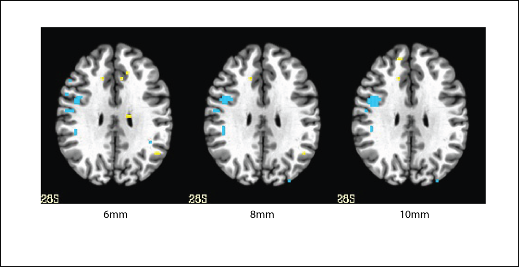
Next we set our spatial smoothing kernel size. If you want to set a FINAL smoothness value, use the -blur_to_fwhm option as well as the line below!
-blur_size 8 \
Next we need to specify where our stimulus timing files are and the condition names. Here I tend to label them c1 and c2, because I later add GLTs to specify the names of the conditions. This is just a style thing for most people doing BLOCK or HRF analysis. But if you are using TENT/CSPLIN, you end up with a series of regressors for each STEP of these functions which can be confusing. You can reduce the confusion by using the condition labels here and the actual names in GLTs which can be used to average over all or part of the window. The final option says that our stimulus timing files are local times, meaning that they are relative to the start of each EPI run. The alternative is global, which would be relative to the start of the first imaging run. I recommend local times, there’s more flexibility if you move things around.
-regress_stim_times stim_times/condition_??.txt \
-regress_stim_labels c1 c2 \
-regress_local_times \
Next we specify the basis function to use. Common options are usually GAM for a gamma function and TENT for making no assumptions about the shape of the HRF and instead estimating it from the data. It’s worth reading the full help of 3dDeconvolve, as there are many other options (SPM with temporal derivative for example) and you should make decisions based on what fits your need or what you’re trying to replicate.
-regress_basis 'GAM' \
The next option is to run the data through 3dREMLfit as well as the normal 3dDeconvolve. The advantage here is that 3dREMLfit includes a correction for temporal correlations via ARMA(1,1). The disadvantage is that it takes a while to run. But on modern computers with multiple CPU cores should be able to accomplish the analyses in only a little more time than using 3dDeconvolve.
-regress_reml_exec \
The next two lines tell afni_proc.py to estimate the smoothness of the data. The first one estimates the smoothness of the input EPIs. The second estimates the smoothness of the error time series file. These values should be roughly comparable, with the errts file being slightly smaller. Take these values in the blur_est.1D files and use them to calculate the inputs of 3dClustSim as shown in my previous post.
-regress_est_blur_epits \
-regress_est_blur_errts \
Next we specify the levels of censoring that the script should use. The first line sets a threshold for outliers of 10% and the second one sets a threshold for motion of roughly 3mm or 3 degrees of rotation (based on euclidean norm).
-regress_censor_outliers 0.1 \
-regress_censor_motion 0.3 \
At this point, almost everything else in the script is directly passed through to 3dDeconvolve or 3dREMLfit. It begins with the line below.
-regress_opts_3dD \
The first options that we pass are that we have 3 contrasts (or GLTs), one for print, one for speech, and one for the subtraction of print-speech.
-num_glt 3 \
-gltsym 'SYM: +c1' -glt_label 1 'print' \
-gltsym 'SYM: +c2' -glt_label 2 'speech' \
-gltsym 'SYM: +c1 -c2' -glt_label 3 'print-speech' \
To speed up processing we include a flag for using multiple processors. This only applies to 3dDeconvolve as 3dREMLfit, 3dAllineate, and a few other programs that are OpenMP enabled will use the max number of threads specified by the environmental variable OMP_NUM_THREADS. You can set this in bash as “export OMP_NUM_THREADS=8”.
-jobs 8 \
Finally we tell afni_proc.py to output the command used to execute the script in bash (my preference), which is really just symbolic as the next line executes the script.
-bash \
-execute
That wraps up a general overview of using afni_proc.py and what each of the options does. There are plenty of other options that one can set, but these are an excellent starting point. I use most of these settings in 90% of the analyses run.


