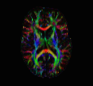
Previously, I talked about how to process DWI/DTI data in FSL and then visualize the results.  AFNI has recently added quite a few tools for analyzing diffusion data.  I’ll cover these in the next post, but first I’ll review correction of eddy currents, coregistering the DWI data to the anatomical and fitting tensors.  The following assumes 1) that you have converted your data via some DICOM converter and eventually ended up with AFNI HEAD/BRIK data files (you can use 3dcopy on your NIFTI files); and 2) that you have DWI data with the b0 image as the first image in your dwi+orig.HEAD file.  The afni.bvecs.txt file is made up of three columns (x,y,z) for your directions in your pulse sequence, there is no line for the b0 image (this is different from FSL!).

If you do not wish to coregister the DWI to high resolution anatomical (I’m sure you have reasons), you can use the alternative “Step 1” as shown below.  Also, while I use the term “Correct Eddy Distortions”, the correct term is more along the lines of “reduce the influence of Eddy Distortions”.  The reason being that they are very hard to model and an Affine transform can only do so much.  

Step 1: Correct Eddy Distortions &
Coregister DWI data to High Res Anatomical Data

align_epi_anat.py -anat anat3d+orig. -epi dwi+orig. \ 
-epi_base 0 -suffix _al2dti -epi2anat \
-giant_move -tshift off -volreg_method 3dAllineate

Step 1 (ALTERNATIVE): Correct Eddy Distortions

3dAllineate -base 'dwi+orig.HEAD[0]' -input 'dwi+orig.HEAD' \
-prefix dwi_al -cost mutualinfo -verb -EPI

Step 2: Fit Tensors using a nonlinear fitting

3dDWItoDT -prefix tensors.nii.gz -automask \
-reweight -verbose 100 -eigs afni.bvecs.txt dwi_al+orig

Step 3: Visualize DTI Data in AFNI

3dcalc -prefix DTIout -a 'tensors.nii.gz[9..11]' -c 'tensors.nii.gz[18]' -expr 'c*STEP(c-0.25)*255*ABS(a)'
3dThreetoRGB -prefix DTIColorMap -anat 'DTIout+orig.[0]' 'DTIout+orig.[1]' 'DTIout+orig.[2]'
afni

Step 3 (Alternative with separate datasets):

3dcalc -prefix DTIout -a 'V1.nii.gz[0..2]' -c 'FA.nii.gz' -expr 'c*STEP(c-0.25)*255*ABS(a)'
3dThreetoRGB -prefix DTIColorMap -anat 'DTIout+orig'

Summary Notes

The first step uses an Affine transform to align all of the different sub-bricks to the first sub-brick (which here is your b0 – e.g. unweighted – image).  If you chose option 1 via align_epi_anat.py, AFNI will also align your DWI data to match your high resolution anatomical.  This is convenient for overlays and also for later warping the DWI data to a standard space (e.g. MNI).  The second step fits our tensors using a nonlinear model – if you wish to use the linear fit (similar to FSL) you can add the -linear flag to the command line of 3dDWItoDT.  The “-reweight” option should also help with some of the distortions introduced in Diffusion Imaging.  The “-eigs” option will compute your eigenvalues, eigenvectors, as well as FA and MD.  Finally, the last step of the Visualize process is to open your DTIColorMap+orig.HEAD in AFNI (see below).  If you open the anat3d+orig as the underlay and the DTIColorMap as the overlay, you will see where the white matter tracts flow through the brain.  In a future post, I will cover the steps involved in deterministic and probabilistic tractography in AFNI as well as some ways to visualize the results.

Diffusion Tensor Map – DEC