Like many scientists, I learned SPSS a long long time ago. It was free and installed on any computer at my undergraduate institution. And like many people, I found the pull-down menus useful and sometimes endearing. But when I went to grad school I was thrust into a world of using SAS. Many a groans were heard in my graduate stats class when we found out that SAS didn’t really have a GUI for doing analyses. But as predicted, I learned to love SAS because it was fast and easy to really delve into your data. Having since used SAS in a production stats environment, I was thankful for how powerful the language was! It turns out the transition to R was even easier than the transition from SPSS to SAS. And it was motivated by three major features 1) R is FREE and SAS is not; 2) R runs natively on a Mac (my computer of choice) and doesn’t require me to run VMWare or Parallel’s Desktop, or better yet lug a PC around with me; 3) R has been extended through the use of many many packages in the community to do everything I could need, and a few things I didn’t know I needed like linear support vector machines (SVM) or random forest “machine learning”.
Between teaching my courses, running some R specific workshops, and doing some consulting work, I’ve been spending a lot of time using R as of late. And so naturally it follows that I now take the time to describe how I use R with AFNI. As I’ve already posted about, you can use R to access AFNI data and perform stats directly on the 3D/4D brain images. But the vast majority of people just want to pull out their Regions of Interest (ROIs) and plot them. This post is for you.
To start, we usually want to get our data into a format that R can handle, for that I use 3dROIstats. Simply supply it a mask and a set of datasets, don’t forget to use your wildcards (*) to make life easier.
3dROIstats -mask ../ROI/final/L_MFG_anterior.nii.gz *.HEAD
This command will output something akin to what is shown below, with information on your file, the sub-bricks in each file, and the value. In this case I have two conditions, print and speech and so each participant is repeated twice in a row.
File Sub-Brick Mean_1
tb1234+tlrc.HEAD 0[print#] 0.060797
tb1234+tlrc.HEAD 1[speech#0_] 0.075399
tb5678+tlrc.HEAD 0[print#] 0.086812
tb5678+tlrc.HEAD 1[speech#0_] 0.011197
To read in you have to realize that R will stop reading after the # unless you tell it to not use the # as a comment character. So I tend to read in the data as follows, resulting in a data.frame with three variables: File, Sub.brick, and Mean_1.
thedata = read.table(file.choose(), sep='\t',header=T, skip=0, comment.char ='')
At this point, I like to rename the Mean_1 to be the ROI that I am using:
names(thedata)[3] = 'L_MFG_Anterior"
At this point, I also like to reformat my Sub.brick variable. You could do this by parsing the variable and doing a series of if/else statements. But I really like to take advantage of the format of my data. Because the data always repeats print and then speech, I can just create a new variable called ‘condition’ using the following:
thedata$condition = c('print','speech')
Now to run a t-test, you can use the t.test command with associated output:
t.test( L_MFG_Anterior ~ condition, data=thedata, paired=T)
Paired t-test
data: L_MFG_Anterior by condition
t = 6.0882, df = 83, p-value = 3.399e-08
alternative hypothesis: true difference in means is not equal to 0
95 percent confidence interval:
 0.07174019 0.14135722
sample estimates:
mean of the differences
 0.1065487
Showing us that our conditions significantly differ. Next we want to plot this, which can be done using either base graphics:
boxplot( thedata$L_MFG_Anterior ~ thedata$condition )
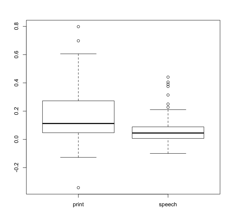
Or my preference using ggplot.
library(ggplot2)
ggplot(thedata, aes(condition, L_MFG_Anterior)) + geom_boxplot() + theme_bw()

Stay tuned for extending this to multiple ROIs and other plot types.