Tips for Remote Processing

Quite a few tools for processing MRI data take considerable amounts of time to run, even with computer hardware getting faster and cheaper daily.  I have previously discussed how to queue up multiple Freesurfer jobs with GNU Parallel in order to automatically queue and dispatch a number of Freesurfer processes simultaneously.  But what do you do if you’re working remotely?  Quite a few people might consider driving into the office just to start the next batch of processing, but hopefully after reading this post, you won’t feel compelled to visit the office just to start more processing!

It’s likely that you’ve at least heard of the first two options (VNC and SSH), but I’ve found that the third option (Screen) is less common and most people haven’t heard of nohup, perhaps because it’s “old school”.

Remote Screen Sharing / VNC

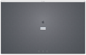
Remote Screen sharing (Mac), remote desktop connection (Windows), or VNC (Mac, Linux, Windows) allows you to view your desktop as if you were sitting directly in front of the computer.  This is particularly useful because it’s like bringing your computer home with you!  If you have a Mac, you can simply turn on Screen Sharing in System Preferences –> Sharing.  If you want to connect to the Mac from computers running other operating systems (e.g. Linux), be sure to click where it says “Computer Settings” in the sharing “control panel” and select VNC Viewers may connect…  Set a good password!  Now to connect to your remote computer you can launch Screen Sharing from the finder (/System/Library/CoreServices/Screen Sharing).  I like to put a copy of the application in my Dock.  When it asks you what to connect to, simply enter the IP address of your work computer.  At some places you may need to setup VPN access, ask your local IT person.  Once you connect, you should see your desktop or login window (below).

VNC


If you are running Linux, I recommend using apt-get, yum, or another package manager (e.g. emerge for Gentoo) to install VNC.  For most major linux distributions, the VNC Client that you use to view another computer is separate from the VNC Server that you use to share your desktop to others.  You can often use the package manager to install both and configuration is often fairly straightforward.

Secure Shell  (SSH)

SSH is a method of connecting via the command line.  The command line is nothing new to most people using MRI software, but you may not have connected to another computer using the terminal or “console” (different terminology).  The upside to SSH is that it uses relatively little bandwidth compared to VNC/Screen Sharing so that you can connect and get real work done, even with a slow network connection.  To turn on SSH on the Mac, turn on “Remote Login” in System Preferences –> Sharing.  Then connect via:

ssh username@ip.address.or.dns.name

Replace the IP address or DNS name with the appropriate value for your computer.  The system will ask for your password and then grant you access to the shell, just as if you had opened Terminal on your own computer.  From here you can see who else is logged on by typing “users” (no quotes) and pressing enter.  You can also see how your processes are doing by typing “top -u” (no quotes).

If you wanted to start a new process, you could do so via SSH just as if you were sitting in front of the computer.  The caveat is that if you close that connection, the process will stop!  And for a process like Freesurfer that takes 12-24 hours, that’s really going to put a damper on things.  So you can either add “nohup” to the beginning of your command which will just append everything to a file called nohup.out, and then close the window, for example:

nohup recon-all -s MySubject -i /path/to/MPRAGE.nii.gz -all -qcache -3T

And if you start a new SSH session, and view top, you will see Freesurfer crunching that brain taking up one processor.  You could of course repeat this or use GNU Parallel alongside nohup to queue your tasks and then close the window.  Either of these should work well for you.  But there’s on other alternative that is really the entire reason I’m writing this blog post today.

The Screen Utility

The screen utility allows you to essentially start an SSH session and then keep it going even after you have closed the window.  I also like to call Screen the ultimate way to bother your IT systems admin because it will continue to show you logged in, making it harder for the IT staff to know when to reboot a computer.  But here’s how it works.  Start an SSH session into your remote computer and type “screen” (no quotes).  You may not have noticed anything change or you may be greeted by a message about screen.  Press space to get rid of the screen welcome.  Now you’re essentially in a shell inside of screen.  You can use this shell just like any other shell, so  go ahead and start a freesurfer job as if you were sitting in front of the computer:

recon-all -s MySubject -i /path/to/MPRAGE.nii.gz -all -qcache -3T

Now that process is running and you see text going across your screen and you’re feeling good about things.  But you now need to disconnect and you don’t want Freesurfer ot quit.  Well if you just close the connection inside of Screen, everything will keep running.  A cleaner (nicer) way to do this is to use your new Screen commands to detach from that particular instance of the shell.  Type Control+A (this tells Screen you want to talk to it and not to the shell) and now press D (upper or lowercase).  This will detach you from the current shell and your process will keep on running.

The reason to use Screen instead of nohup is that you can reconnect to your remote computer (from any computer) via SSH and pickup your session where you left off.  To do this, SSH back into your work computer and now type “screen -ls” (no quotes) and you will see something like the following:

There is a screen on:
 88057.ttys003.frankenstein (Detached)
1 Socket in /var/folders/ng/zpkm15497dd9d6x2sc96zsbm000c5p/T/.screen.

This shows you that there is one Screen session running on my machine Frankenstein.  To connect to that session you just need the name of the session and call screen with the -r flag.  Like so:

screen -r  88057.ttys003.frankenstein

And now you are reconnected and you should see the Freesurfer output continuing to scroll across the screen (or if you waited long enough perhaps it is done).  If you find this helpful or interesting, you can read more about screen here.  Or use the magical powers of Google.

Summary

So there you have it, three (or more) ways to connect to your work computer to start new processing without having to physically be in front of the computer.  I would say that major advantage of using Screen is that you don’t have to be controlling a remote screen, so people won’t begin to think that their computer is possessed when the mouse just starts moving.  It’s also worth noting that GNU Parallel will work inside of a screen session and that you can pair the two together.  The advantage to using Screen + Parallel is that if you wish to cancel a process, it’s considerably easier than killing Parallel + nohup!
Creating Volume ROIs in AFNI

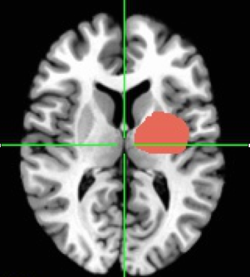
For those keeping track at home, an ROI involves selecting a section of the brain (or subset of voxels) that you have some interest in.  The ROI can be a geometric shape or drawn by hand.  It can be defined by anatomical markers or by functional activation or really by anything you want.

Screen Shot 2013-07-25 at 7.12.59 AM

AFNI has a number of ways of creating Regions of Interest (ROIs), I review some of the more common ways of creating an ROI below.  I will cover creating ROIs on the surface for use with SUMA in a later post!

Draw an ROI by hand

  1. Open AFNI Viewer
  2. Set Underlay as Subject’s Anatomical (anat_final if you use afni_proc.py)
  3. Right Click on Anatomical image in any view (axial, sagittal, coronal)
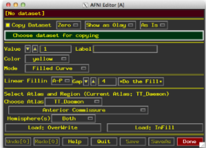
  4. Select Draw ROI Plugin (the window below will appear)
  5. Set your dataset for copying as the anatomical
  6. Select a mode for drawing
    1. Filled Curve lets you click draw freehand style
    2. Sphere and Circle options with size options
    3. Specify a value – if you have more than one ROI, give them different values!
    4. Third Mouse Click on the image where you want the ROI to be (or draw freehand while holding middle click)
    5. When complete, press Save.
  7. Down sample the mask to the size of your stats or functional datasets via 3dresample or 3dfractionize!
  8. Extract values with 3dmaskave, 3dmaskdump, 3dROIstats, etc…

Screen Shot 2013-07-24 at 4.52.38 PM

Create ROI mathematically using coordinate systems

You can create an ROI using 3dcalc.  Example #7 in the help of 3dcalc shows that the following code can be used to create a sphere ROI with a radius of 3 with origin (center) at x=20, y=30, z=70.

3dcalc -a anat+tlrc \
-expr 'step(9-(x-20)*(x-20)-(y-30)*(y-30)-(z-70)*(z-70))' \
-prefix ball

You will need to down sample the ROI for your functional or stats dataset using 3dfractionize or 3dresample.  Then you can extract values with 3dmaskave, 3dmaskdump, 3dROIstats, etc…  You can also draw other shapes fairly easily using 3dcalc.

If you just wish to create a sphere, you can use the -srad option in 3dUndump.  3dUndump also allows you to specify the values of specific voxels from either the terminal or a 1D file or with a combination of 3dmaskdump and 3dUndump (I like to do things with AWK or Python in the middle of the dump and Undump).

Create ROI from functional activations

  1. Load underlay as your subjects anatomical (anat_final if you use afni_proc.py)
  2. Load overlay as your subjects stats file (REML if you like)
  3. Set OLay and Thr sub-briks to your coefficient and t-stat (or t-stat for both if you’re inclined!)
  4. Set p-value to a value you feel is appropriate
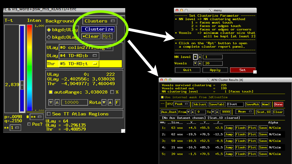
  5. Turn on Clustering using the Clusterize button
  6. Specify a Cluster size (can use a value you like or one from 3dClustSim)
  7. Click Set and then Click “Rpt” for “Report”
  8. See a window listing the clusters that meet threshold and your criteria for size.
    1. Play around with Jump, Flash, Plot (need AUX dataset set), and Save
    2. Notice that list of clusters changes as you change the p-value using your t-stat slider!
  9. To Save Clusters press “SaveMsk”, see a 3dClust command presented in the terminal.
  10. Notice automatically created Clust_mask+tlrc.HEAD/BRIK
  11. Each cluster saved with a separate value 1 to X, where X is the max number.
  12. Extract values for 2nd largest cluster via: 3dmaskave -mask Clust_mask+tlrc.HEAD'<2>’ mydataset+tlrc.HEAD
  13. Extract all/other values with 3dmaskave, 3dmaskdump, 3dROIstats, etc…

functional_roi

Create ROI based on Atlas defined anatomical region

  1. Identify which Atlas you wish to use, full list seen in: whereami -show_atlases
  2. Identify which regions are available in the Atlas you have chosen: whereami -show_atlas_code -atlas CA_N27_ML
  3. Create a mask for region of choice: whereami -mask_atlas_region CA_N27_ML:left:middle_frontal_gyrus -prefix left_mfg
  4. Repeat with other regions if necessary
  5. OPTIONAL: combine into single mask: 3dcalc -a left_mfg+tlrc -b right_mfg+tlrc -prefix mfg_lr -expr ‘1*a + 2*b’
  6. Down sample the ROI to your functional or stats datasets with 3dresample or 3dfractionize
  7. Extract values with 3dmaskave, 3dmaskdump, 3dROIstats, etc…

Create ROI based on individual subject Freesurfer Segmentation

  1. Run freesurfer segmentation for your participant
  2. Navigate to that folder in Terminal/Shell and run @SUMA_Make_Spec_FS
  3. cd into the SUMA directory
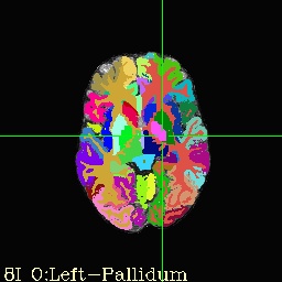
    1. If you launch AFNI, set underlay as brain.nii and overlay as aparc+aseg_rank or aseg_rank for same visualization as below!
  4. Identify region of interest in one of the following NIML label tables
    1. aparc+aseg_rank.niml.lt
    2. aparc.a2009s+aseg_rank.niml.lt
    3. aseg_rank.niml.lt
  5. Create ROI: 3dcalc -a aseg_rank.nii'<15>’ -prefix L_AMG.nii.gz -expr ‘step(a)’
    1. Creates subject specific ROI in Left Amygdala
  6. Make sure this is aligned the same as your anat_final dataset
  7. Down sample to your functional or stats dataset using 3dresample or 3dfractionize
  8. Extract values with 3dmaskave, 3dmaskdump, 3dROIstats, etc…

temp

Summary

Are you tired yet?  As you can see there are a significant number of ways to make ROIs in AFNI.  I will cover the options for getting data out of ROIs in a later post.

Analyzing DTI Data in AFNI (Part 1)

Previously, I talked about how to process DWI/DTI data in FSL and then visualize the results.  AFNI has recently added quite a few tools for analyzing diffusion data.  I’ll cover these in the next post, but first I’ll review correction of eddy currents, coregistering the DWI data to the anatomical and fitting tensors.  The following assumes 1) that you have converted your data via some DICOM converter and eventually ended up with AFNI HEAD/BRIK data files (you can use 3dcopy on your NIFTI files); and 2) that you have DWI data with the b0 image as the first image in your dwi+orig.HEAD file.  The afni.bvecs.txt file is made up of three columns (x,y,z) for your directions in your pulse sequence, there is no line for the b0 image (this is different from FSL!).

If you do not wish to coregister the DWI to high resolution anatomical (I’m sure you have reasons), you can use the alternative “Step 1” as shown below.  Also, while I use the term “Correct Eddy Distortions”, the correct term is more along the lines of “reduce the influence of Eddy Distortions”.  The reason being that they are very hard to model and an Affine transform can only do so much.  

Step 1: Correct Eddy Distortions &
Coregister DWI data to High Res Anatomical Data

align_epi_anat.py -anat anat3d+orig. -epi dwi+orig. \ 
-epi_base 0 -suffix _al2dti -epi2anat \
-giant_move -tshift off -volreg_method 3dAllineate

Step 1 (ALTERNATIVE): Correct Eddy Distortions

3dAllineate -base 'dwi+orig.HEAD[0]' -input 'dwi+orig.HEAD' \
-prefix dwi_al -cost mutualinfo -verb -EPI

Step 2: Fit Tensors using a nonlinear fitting

3dDWItoDT -prefix tensors.nii.gz -automask \
-reweight -verbose 100 -eigs afni.bvecs.txt dwi_al+orig

Step 3: Visualize DTI Data in AFNI

3dcalc -prefix DTIout -a 'tensors.nii.gz[9..11]' -c 'tensors.nii.gz[18]' -expr 'c*STEP(c-0.25)*255*ABS(a)'
3dThreetoRGB -prefix DTIColorMap -anat 'DTIout+orig.[0]' 'DTIout+orig.[1]' 'DTIout+orig.[2]'
afni

Step 3 (Alternative with separate datasets):

3dcalc -prefix DTIout -a 'V1.nii.gz[0..2]' -c 'FA.nii.gz' -expr 'c*STEP(c-0.25)*255*ABS(a)'
3dThreetoRGB -prefix DTIColorMap -anat 'DTIout+orig'

Summary Notes

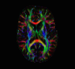
The first step uses an Affine transform to align all of the different sub-bricks to the first sub-brick (which here is your b0 – e.g. unweighted – image).  If you chose option 1 via align_epi_anat.py, AFNI will also align your DWI data to match your high resolution anatomical.  This is convenient for overlays and also for later warping the DWI data to a standard space (e.g. MNI).  The second step fits our tensors using a nonlinear model – if you wish to use the linear fit (similar to FSL) you can add the -linear flag to the command line of 3dDWItoDT.  The “-reweight” option should also help with some of the distortions introduced in Diffusion Imaging.  The “-eigs” option will compute your eigenvalues, eigenvectors, as well as FA and MD.  Finally, the last step of the Visualize process is to open your DTIColorMap+orig.HEAD in AFNI (see below).  If you open the anat3d+orig as the underlay and the DTIColorMap as the overlay, you will see where the white matter tracts flow through the brain.  In a future post, I will cover the steps involved in deterministic and probabilistic tractography in AFNI as well as some ways to visualize the results.

dti_dec1

Diffusion Tensor Map – DEC


Basics of AFNI Group Analyses (Part 2)

So after last time, you successfully ran a group-level analysis that you feel fits your scientific question and now you want to know what will survive statistical scrutiny. Well the good news is that you have a few options! First, in order to get any of these options working, you should start by running your group-level analysis with a mask to remove activity outside of the brain (yes it still happens). Since we need the mask to consider which statistical correction to apply, let’s start there.

Generating Masks for Group Level Analysis

Just in terms of generating a group-level mask, you have a few options. If you’re using afni_proc.py (which I highly recommend), and you warp your data to standard space early on (e.g. -volreg_tlrc_warp), you can get a file from each subject called mask_group+tlrc.HEAD, which is the individual subjects brain mask after being warped to standard space. You can collect these from each subject and then average them via 3dMean. This can be helpful also to look at registrations as a whole!

If you didn’t use afni_proc.py, then you can take each subject’s standardized anatomical data (without skull) and run 3dAutomask on the brain (default settings tend to work). You can then take all of these and use 3dMean to put them together to create your group mask. Note that the opposite approach will give you similar results, running 3dMean on all of your subject anatomicals in standard space and then using 3dAutomask on that average.

Your third option is to take the standard space anatomic (e.g. TT_N27 or MNI152) and mask that for use with your group analysis. The warning here is that registrations are usually not perfect, so you could be masking out important bits of data from some subjects.

Whether you chose options 1, 2, or 3, it’s possible that your mask is a different size (different dimensions) from your statistical datasets. You can verify this by running 3dinfo -prefix -d3 -n4 *.HEAD in a folder containing all of your stat files and your mask. If your mask turns out to be a different size than your stats datafiles, you can use either 3dresample or 3dfractionize to reduce the size of your mask to match your stats datasets.

Statistical Corrections

Now that you have a group mask, you can re-run your data analysis using whatever group program you used before (e.g. 3dttest++, 3dANOVAx) and you will automatically get a “free” FDR correction for each of your comparisons that no longer takes into account all the voxels way outside of the brain. This will allow you to see in the viewer an associated FDR “q-value” for each t-value and p-value that you are used to looking at.

But ultimately, FDR has plenty of things that people don’t like about it, the first of which is that it can make statistical results disappear, even when you have large “blobs” or activation in your group level analysis. The major alternative in AFNI is to use cluster-wise thresholds, where clusters of a large number of voxels count as surviving statistical scrutiny. The way that this is implemented in AFNI is through 3dClustSim.

Before running 3dClustSim, you need to estimate the blur for each of your datasets. If you used afni_proc.py (or uber_subject.py), you can grab the file blur_est.${subject_number}.1D for each subject and average the values (x,y,z) labeled “errts blur estimates” and get your overall group-level blur level to input into 3dClustSim. If you don’t use afni_proc.py, you can run 3dFWHMx on each of your errts datasets with your subject level mask and use those numbers in an average.

Finally, now that you have a Group level mask and your average blur size, you can run 3dClustSim to generate the necessary cluster size for a given p-value to survive statistical correction. Substitute the 9 9 9 for your actual average blur in the example below. This is highly derived example, typical cluster sizes are much larger than those shown below (in part because your datasets are at a higher resolution).

3dClustSim -mask mask+tlrc -fwhmxyz 9 9 9 -niml -prefix CStemp
# 3dClustSim -fwhmxyz 9 9 9
# Grid: 64x64x32 3.50x3.50x3.50 mm^3 (131072 voxels)
#
# CLUSTER SIZE THRESHOLD(pthr,alpha) in Voxels
# -NN 1  | alpha = Prob(Cluster >= given size)
#  pthr  |  0.100  0.050  0.020  0.010
# ------ | ------ ------ ------ ------
 0.020000   112.3  125.0  142.6  154.9
 0.010000    69.5   77.9   89.0   96.7
 0.005000    47.5   53.3   62.1   68.1
 0.002000    31.7   35.9   41.3   45.8
 0.001000    24.2   27.9   32.4   36.0
 0.000500    19.0   21.9   25.7   29.0
 0.000200    14.1   16.5   19.8   22.3
 0.000100    11.4   13.4   16.3   18.4

This table shows on the left a p-value and to the right the necessary cluster size for a given alpha level.  So if you want an alpha of 0.01, you need a cluster of 154.9 voxels at p=0.02.  You can also embed this information into the output of your group analysis program so that when you view the results in AFNI, you can see a p-value associated with each cluster given a set t-value.  The most amazing part of this is that the AFNI viewer will update your clusters on the fly.

3drefit -atrstring AFNI_CLUSTSIM_NN1 file:CStemp.NN1.niml \
 -atrstring AFNI_CLUSTSIM_MASK file:CStemp.mask \
 statistics_dataset+tlrc


Basics of AFNI Group Analyses (Part 1)

I’ve been working on quite a few things recently, and will get back to regular posts soon.  In the meantime, here’s a brief introduction to Group Analysis tests in AFNI.

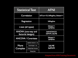
I see the information related to Group Analyses falling into two categories: 1) Which program to run and when; 2) all the other stuff related to Group Analyses beyond just running one program to compare X.  Today I’m going to outline the programs one would use for doing different types of Group (sometimes also called 2nd-level) analyses.  To aid this, I’ve adapted an AFNI table and attached it below.

analysis


As you can see, for just about any type of group level test, there exists one (and sometimes MANY) different AFNI programs.  The choice of which program to use can depend on what you’re already comfortable with or what you really need for a particular analysis.  For example, you can use 3dRegAna to do regression, or ANCOVA.  But an easier way to do an ANCOVA is to use 3dttest++ or 3dMEMA because in 3dRegAna you must specify each variable in the command; whereas in 3dttest++/3dMEMA you can use a text file to list out your covariates and have them all run simultaneously to view the impact of each covariate on your model.

Another reason to choose one program over another is speed.  You can perform ANOVAs (one-way or multi-factorial) in 3dANOVA (and it’s cousins 3dANOVA2 and 3dANOVA3), or you can do this same analysis in 3dMVM (MVM = Multivariate Modeling).  The advantage of 3dANOVA/2/3 is speed, these programs run incredibly fast!  The disadvantage of 3dANOVA/2/3 is that they require balanced designs (no unequal groups) and they cannot take covariate information.  In swoops 3dMVM, which can handle both unbalanced designs and covariates, but is considerably slower.

I will also take a moment and recommend that everyone look through the help information on gen_group_command.py, which can automatically generate the necessary commands for 3dttest++, 3dMEMA, 3dANOVA, 3dANOVA2, and 3dANOVA3 based on the input files (passed to the script) and some additional information, which can be a huge time saver.

gen_group_command.py -command 3dttest++ \
 -write_script ttest_example.tcsh \
 -prefix condition_${name}.nii.gz \
 -dsets subject??.nii.gz \
 -subs_betas 'conditionA#0_Coef'

Just that will generate a script to run 3dttest++ (saved to ttest_example.tcsh).  That script will run a single-sample t-test on the data files in the folder that are labeled subjectXX.nii.gz, where XX are two numbers, for a particular condition.  In addition to being a huge time saver for generating one script, this is also very helpful for allowing you to quickly add or remove subjects to the t-test (please use statistics responsibly!).