Basics of DTI Analysis (FSL)

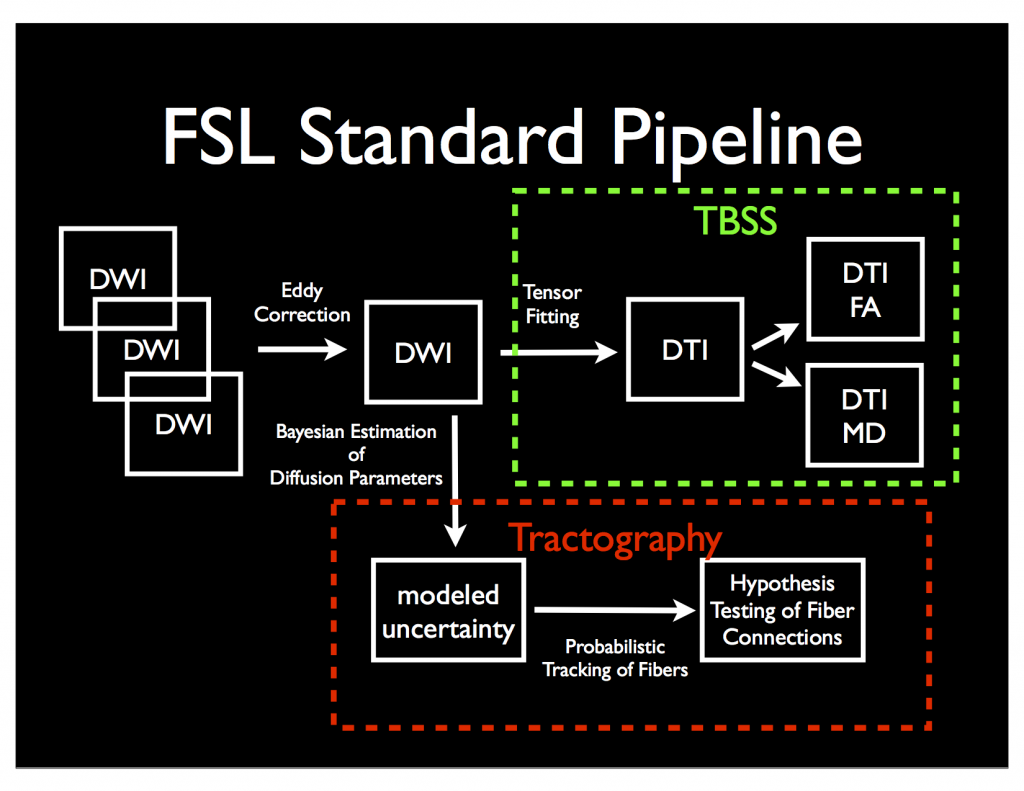
FSL has a complete pipeline for converting Diffusion Weighted Images (DWI) to Diffusion Tensor Images (DTI) using one of two pipelines: 1) “Tract-Based Spatial Statistics” or 2) Probabilistic Tractography (via Bedpostx and probtrackx).  The graphic below shows a rough overview of each.

DTI


The analysis with FSL is fairly straight forward.  If you wish, you can run the FSL Diffusion Toolkit via the Graphical User Interface (GUI) by typing FSL and then clicking FDT or by launching FDT directly – type Fdt_gui into the terminal on a mac, or omit the “_gui” on linux.  Alternatively you can process the data via the command line, which ends up being easier to batch across multiple subjects!  I’ll print the command lines below along with a step by step guide.  We’ll start with the TBSS pipeline and I’ll save the bedpostx and probtrackx for another post.

Step 0: Organize all of your subjects into consistent naming schemes and into separate folders.  If you used dcm2nii to convert your DICOM files to NIFTI format, it will conveniently also generate a bvec and bval file for each DWI NIFTI file.

Step 1: Eddy Correction

eddy_correct subject1.nii.gz subject1_ec.nii.gz 0

Step 2: Create Mask – necessary for tensor fitting!

bet subject1_ec.nii.gz subject1_ec_mask.nii.gz -m -n -R

Step 3: Fit Tensors

dtifit -k subject1_ec.nii.gz -o subject1_tensor.nii.gz -m subject1_ec_mask.nii.gz -r subject1.bvec -b subject1.bval -V

Step 4: TBSS Preprocessing

More detailed instructions available from FSL Wiki!

First, copy all of your FA files into one folder.  Next, take a look at your data files, I recommend naming them in a way that the groups stick together.  Perhaps adding a prefix of “Control_” to one group and “Exp_” to the other.  Use design_ttest2 to layout your design.mat and design.con files.

Next, run tbss_1_preproc *.nii.gz inside that folder.  Followed by tbss_2_reg to register all images to the template.  tbss_3_postreg will actually apply the nonlinear registration.  tbss_4_prestats will threshold the images.  Finally you can use randomise to run your analyses.
Quality Checking fMRI

You can never be too careful in terms of data quality.  AFNI offers a number of checks on the data via the automated @ss_review_basic and @ss_review_driver generated by afni_proc.py.  But occasionally you need more information!  And also if you’re comparing data across multiple scanners, it’s not a bad idea to have some of these numbers for doing just that!  It’s also worth noting that the fBIRN utilities can also be useful for processing phantom data for comparing between scanners.  But really, this post is about how to get these QC/QA checks working!  Installing the fBIRN QC/QA tools on a Mac requires a little bit of hackery!

  1. Install AFNI.  I feel like most people already know that would be step 1 if you’re reading this blog.
  2. Install Xcode for Mac OS X
    1. If running 10.7 or later, use the App Store
    2. If running 10.5/10.6, either install off the CD or head to Apple Developer
  3. Head over to the BIRN site and grab the xcede tools (alternatively go straight to nitrc).
    1. Install the tools into a convenient directory (e.g. /usr/local/xcede)
    2. Add /usr/local/xcede to your path
  4. Install homebrew – you won’t regret it
    1. Homebrew is a package management system for installing (mostly) unix/linux tools.
    2. Run this to install: ruby -e “$(curl -fsSL https://raw.github.com/mxcl/homebrew/go)”
  5. Install a few brew packages
    1. brew install imagemagick
    2. brew install ghostscript
  6. Remove copies of the BIRN tools that don’t work on mac
    1. cd /usr/local/xcede/bin
    2. rm convert
    3. rm montage
  7.  Link the homebrew installed tools to where you removed the old tools!
    1. ln -s /usr/local/Cellar/imagemagick/6.7.7-6/bin/convert /usr/local/xcede/bin/convert
    2. ln -s /usr/local/Cellar/imagemagick/6.7.7-6/bin/montage /usr/local/xcede/bin/montage
  8. Change into a directory with a NIFTI file for testing
    1. cd /path/to/MRIdata
  9. Test it out!
    1. Convert to XML: analyze2xcede aNiftiFile.nii.gz QA_aNiftiFile.xml
    2. fmriqa_generate.pl QA_aNiftiFile.xml QADirectoryName
    3. Repeat for each run in your subject and for all subjects!

This will generate an output folder with a series of files inside.  Open up the index.html file for the main report.  In particular, pay attention to the SNR and SFNR values.  If these are low (less than 40, you should be concerned!).  It could be that you need to crop off the first few pre-steady-state images before running the script.  Alternatively you can run fmriqa_generate.pl with the –timeselect 4: flag to not process the first four TRs.  Read the help for more info!

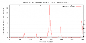
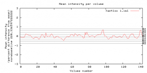
There are also a series of helpful charts for seeing if things went wrong.  Below are just two of the many many helpful charts generated automatically.  The first shows outliers (output of 3dToutcount from AFNI) and the second shows mean intensity per volume.

qa_outliercount_allqa_volmeans_all

Source Code Available

Some time ago, I made available a series of custom-built software packages for helping perform EEG/ERP Analysis.  I have now finished uploading the source code to my github repository.  All of the programs were written in Objective-C, many of them fairly early in my programming career (forgive the comments or lack of comments!).  If you find them helpful, please drop me a line at peter (at) cogneurostats.com!

Using R with AFNI

AFNI already has a host of programs that use R to analyze MRI data – 3dLME, 3dMVM, 3dMEMA, etc.  Suppose you wanted to create your own functions that use R to manipulate data – well here’s a quick introduction.  In this quick example, here is how to “Auto Mask” your dataset in R.

source('path/to/AFNI/AFNIio.R')
thedata = read.AFNI('run1+orig')
names(thedata)

#get value at voxel at time point
#here midpoint x, y, z, time point 66
thedata$brk[32,32,10,66]
testdata = thedata$brk[,,,1]
for ( i in 1:dim(testdata)[1] ) {
   for ( j in 1:dim(testdata)[2] ) {
      for ( k in 1:dim(testdata)[3] ) {
         if( testdata[i,j,k] > 400 ) {testdata[i,j,k] = 1;}
         else {testdata[i,j,k] = 0;}
       }
    }
}
write.AFNI("test_mask+orig", brk=testdata, label=NULL, note="Masked", orient=thedata$orient, view='+orig', defhead=thedata$header)

I take some shortcuts by just making the output dataset header identical to the input dataset.  But you get the general sense for how easy it is to open an AFNI dataset in R, manipulate the data and write it back out.

A better way to run AFNI’s uber_subject

I used to use fink, and then I switched to MacPorts; truthfully, neither of them really made me happy.  Now I mostly use homebrew, and one real advantage (besides being faster and lighter weight) is that it’s very easy to get AFNI’s GUI programs up and running on a Mac.

  1. Install AFNI (you’ve probably already done this)
  2. Install Xcode (App Store)
  3. Install Homebrew
    1. ruby -e “$(curl -fsSL https://raw.github.com/mxcl/homebrew/go)”
  4. Install PyQT
    1. brew install pyqt
  5. Set Python Path
    1. export PYTHONPATH=/usr/local/lib/python2.7/site-packages:$PYTHONPATH
    2. Consider adding the above line to your .bashrc or .profile (assuming Bash Shell)
  6. Run any AFNI uber_*.py programs
    1. uber_subject.py
    2. uber_ttest.py
    3. uber_align_test.py