I think we’ve all had that moment where we wonder what exactly our HRF function is doing to give us the results that we see in our data.  Using a fixed function regressor can be great for a number of reasons: 1) they don’t require many degrees of freedom, 2) someone else did the hard work to figure them out, 3) they often do a pretty good job of modeling the hemodynamic response that has been well documented.  Yet every so often we want to know what the actual response looks like, either to double check our Gamma function style HRFs or possibly because we’re interested in aspects of the shape of the actual response.  Consider this a quick introduction to some options you have when using TENT functions for estimating the shape of the blood flow response directly from the data.

First and foremost, it’s not always necessary to go back and rerun all of your data (including preprocessing) using a new afni_proc.py script.  Instead you can use a modified script to just take your already preprocessed data and run only the regression step (see how here).  Great, well that just saved you a ton of time, so head over to the 3dDeconvolve 2004 upgrades page and take a peek at some of the “newer” possibilities.

Basic TENTs

Now that you’ve read that, let’s take a quick second to look at some of the essential parts of our afni_proc.py (or 3dDeconvolve) options.  First and foremost you have your actual definition of the TENT function, which usually goes something like:

-regress_basis 'TENT(0,12,7)'

Here I’m asking 3dDeconvolve to estimate the response starting at the stimulus onset (0 seconds) and estimate out to 12 seconds.  Since I have a TR of 2 seconds, that means that there are 7 possible TENTs to fit during this time.  When you do this, 3dDeconvolve will generate a Coef and Tstat for EACH and EVERY TENT that you requested.  This isn’t always terribly useful since you may not really care what the “area under the curve” is for say TENT #5 independent of everything else.  Fortunately, you can use the GLT system to get the average over all of these TENTs:

-gltsym 'SYM: +1*conditionA' -glt_label 1 'ConditionA'

Displaying TENTs in AFNI

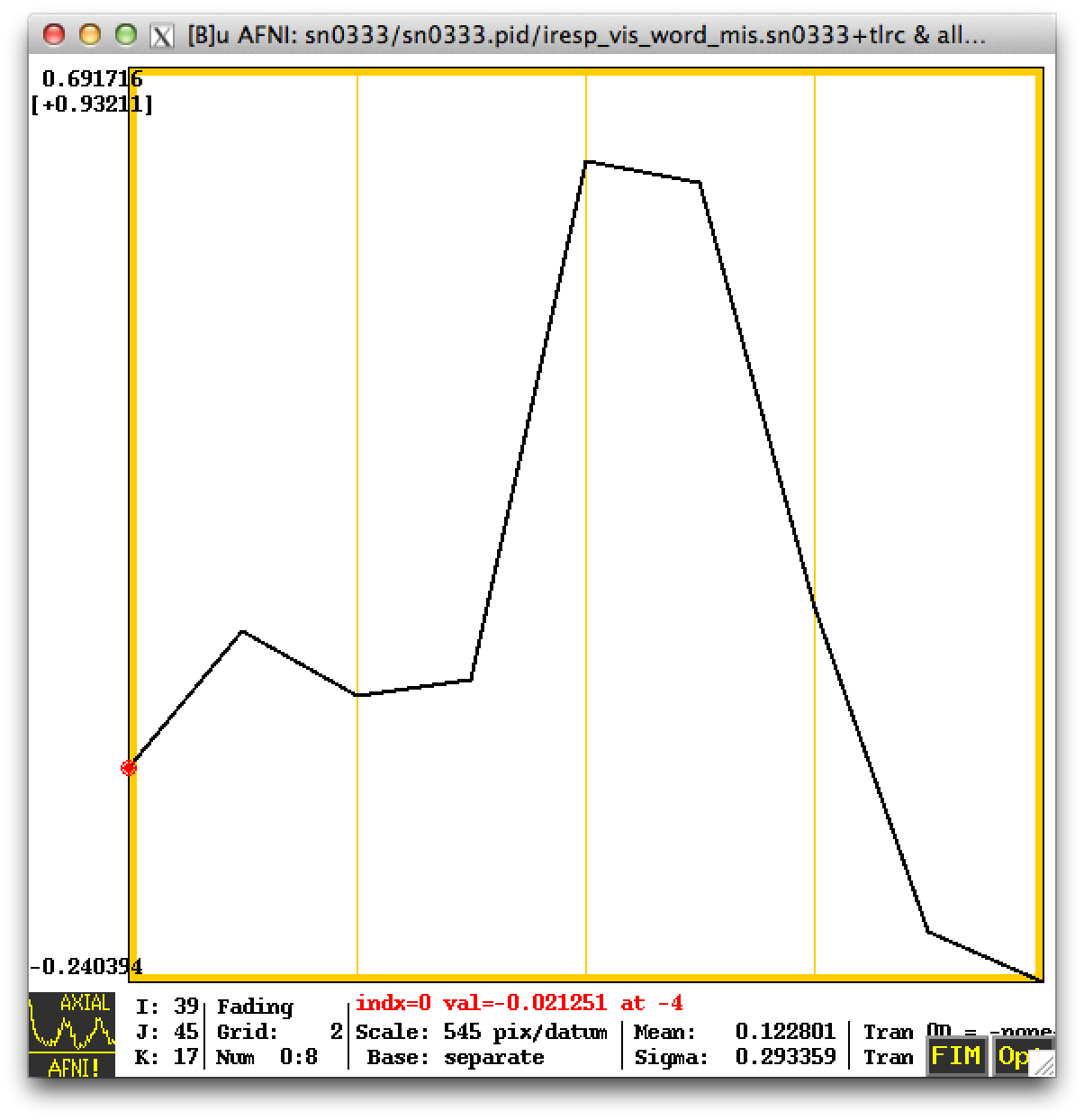
Once you’ve run an analysis with TENT, you can visualize the TENT at any voxel within the AFNI viewer using the following steps.

1. Open AFNI viewer, set underlay as your anatomical
2. Optionally you can set the overlay to the stats dataset and select your GLT as described above.  This will show you were there is activation according to the model, which may help inform your selection of a voxel to visualize.
3. Open a new AFNI viewer (press the New Button) and make the following selections
   1. Set underlay as the iresp file representing your condition of interest
   2. Click the graph button
4. At this point, moving around on the statistical dataset will show you what the associated response looks like for that particular location.

Other TENT Possibilities

If you want to force your first and last time points in the TENT to be zero, you can use the TENTzero function instead of TENT.  This might be useful.  Ok, it is useful.

Alternatively, if you like the idea of ERPs using peak measures, you might want to contrast the “peak” of your response to the “baseline” or pre-stimulus intervals.  In order to do this, you should tell 3dDeconvolve to use TENT to model some of the time series BEFORE the onset of a stimulus as so:

TENT(-4,12,9)

Here we ask 3dDeconvolve for 4 seconds before the onset of the stimulus and extending to 12 seconds after the stimulus, using 9 TENTs.  In this case, you may not want to use the same GLT you did before, because it would include the pre-stimulus time in the average.  So you can use square-brackets to index one or several TENTs:

-gltsym 'SYM: -1*conditionA[0..2] +1*conditionA[4..6]' -glt_label 1 'conditionA_Peak'

Here we’re subtracting the first 3 TENTS (0, 1, 2) from what I’m calling the “peak” TENTS (4, 5, 6).  Now it’s important to recognize that TENT 0 is -4 seconds, TENT 1 is -2 seconds, TENT 2 is at 0 seconds relative to stimulus onset.  Continuing on TENT 3 is at 2 seconds, TENT 4 is at 4 seconds, TENT 5 is at 6 seconds, and TENT 6 would be at 8 seconds.  So we’re subtracting activations 4 seconds before the stimulus onset from activations 4-8 seconds after.

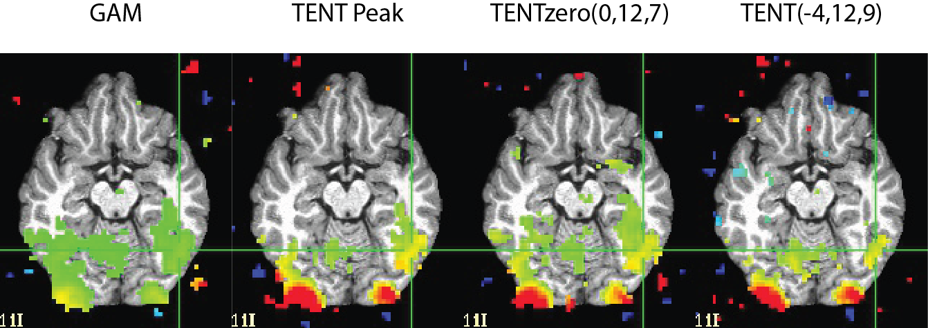
But how much of a difference does it really make?  Well, of course this is fMRI, so the answer is “it depends”.  If we look at the response curve shown at the top of the article, you might recognize how close it looks to the Gamma function.  If we compare the resulting maps on a basic in-scanner reading experiment, you can see the Gamma shows the most activation; TENTzero over a 12 second window and “TENT Peak” where I pull out the peak (4-8 seconds) and subtract the pre-stimulus interval are fairly close in activation.

I also included the map for the average over both the pre-stimulus and post-stimulus interval to illustrate that you want to be careful NOT to accidentally include the entire window if you have the pre-stimulus baseline included as it may reduce the activations of interest.