Basics of AFNI Group Analyses (Part 3)

It’s been a while since I’ve touched on this topic (Part 1, Part 2).  Recently the topic of doing t-tests has come up a lot in the area around where my desk is situated.  In vastly over simplified thinking, I think the three most common approaches to using t-tests in MRI data are as follows:

  1. One-sample t-test – identify significant activation exists compared to zero.
  2. Two-sample t-test – identify where two groups differ in activation
  3. Paired-sample t-test – identify where two conditions differ

It’s important to note that these group level t-tests can be performed on single activation coefficients or on contrasts at the single subject level.  Be careful, this can get complicated very quickly if you’re asking for how two groups differ on a difference between two conditions.  Avoiding for a moment the hot debate about correct statistics to use, let’s just focus on using 3dttest++ via gen_group_command.py to perform these three analyses.  For anyone not yet familiar with gen_group_command.py, it is a python script that easily generates syntax to run 3dttest++, 3dMEMA, 3dANOVA2, and 3dANOVA3.  It’s well worth learning!  That said, for the examples in this post, I have a dataset where participants either read print in the scanner or listened to speech.

In order to get the subs_betas used below, I ran 3dinfo -verb subject01+tlrc. and found that I had Coef (stands for coefficients) for print and speech with the format ‘print_GLT#0_Coef’ ‘speech_GLT#0_Coef’, I could also use the numbers corresponding to those sub-briks, but I think using names is safer and would encourage you to do the same!  I’ve also included the -set_labels command, which will label the output sub-briks in useful ways for interpreting the analyses later on!

One-sample t-test

If I wanted to see what areas of the brain activate in response to one of these conditions, I would choose to do a one-sample t-test.  For example using just print, the gen_group_command would look something like this:

 gen_group_command.py -command 3dttest++ \
 -write_script ttest_print.tcsh \
 -prefix print_results \
 -dsets subject??.stats+tlrc.HEAD \
 -subs_betas print_GLT#0_Coef \
 -set_labels print

If I wanted to look at the difference between print and speech, I could also use a one-sample t-test, if I thought ahead and included that GLT in the single subject analysis.  It would look something like this:

 gen_group_command.py -command 3dttest++ \
 -write_script ttest_print-speech.tcsh \
 -prefix print-speech_results \
 -dsets subject??.stats+tlrc.HEAD \
 -subs_betas print-speech_GLT#0_Coef \
 -set_labels print-speech

Paired-sample t-test

If I didn’t think ahead and put the print-speech contrast in the single-subject analysis, I could instead use a paired-sample t-test (because they are the same subjects).  Notice the two separate Coef’s in the subs_betas line and the two uses of the -dsets option!

 gen_group_command.py -command 3dttest++ \
 -write_script ttest_print-speech.tcsh \
 -prefix print-speech_results \
 -dsets subject??.stats+tlrc.HEAD \
 -dsets subject??.stats+tlrc.HEAD \
 -subs_betas print_GLT#0_Coef speech_GLT#0_Coef \
 -set_labels print speech \
 -options -paired

Two-sample t-test

Now if I had two groups of subjects and I wanted to look at how those two groups differed on brain responses to print, I would use a two-sample t-test.

 gen_group_command.py -command 3dttest++ \
 -write_script ttest_print-speech.tcsh \
 -prefix print-speech_results \
 -dsets Group1/subject??.stats+tlrc.HEAD \
 -dsets Group2/subject??.stats+tlrc.HEAD \
 -subs_betas print_GLT#0_Coef \
 -set_labels print

Don’t forget to run the scripts!

It’s important to note that running gen_group_command.py just sets up the script for you.  Here my individual subject files are labeled subject01, subject02, etc.  You can look at the generated tcsh script and make sure that the command looks something like what you wanted.  Then you can execute the script by typing: tcsh MyScript.tcsh, where “MyScript.tcsh” is one of your t-tests that you created with gen_group_command.py.

Don’t forget you can mask too!

Masking allows us to hide activation outside of where we might want it.  But while it makes pretty pictures, it can also cause you to miss problems in your data.  When I first run group analyses, I usually don’t mask the data, this allows me to see if there are glaring problems (like huge activation outside of the brain).  With any of the snippets above, you can pass gen_group_command.py the flag -options and after that a -mask and the path to your mask.  You could easily run the gen_group_command.py twice, once with and once without the mask.  As an alternative, you could mask the data after the fact using 3dcalc.

3dcalc -a print-speech_results+tlrc -b MyMask+tlrc -expr 'a*b' -prefix masked_print-speech_results

I always put the dataset first and the mask second, because 3dcalc will by default output a dataset in the same datum (float, byte, short) of the first dataset passed to it.  Try switching them and you’ll be greeted by a warning and data that doesn’t look the way you think it should!
 

Single Subject Analysis on the Surface (SUMA)

I had previous posted about displaying the fMRI results onto the cortical surface.  It’s been brought to my attention that this post wasn’t as clear as it could be!  I know, it happens from time to time!  So let’s try this again!  Let’s start with a straightforward topic – processing data at the single-subejct level on the cortical surface.  There are a variety of reasons that you might want to do this!

  1. Surface-based registration methods are likely superior to volume registrations
  2. Surface-based analysis allows you to smooth along the surface, which is better.
  3. Surfaces look pretty
  4. And many others…

Generate Cortical Surfaces

First thing is first.  You generate your cortical surfaces using Freesurfer, BrainVoyager, Surefit, Caret, or rumor has it BrainSuite.  I have the most experience using Freesurfer, so for the purposes of this post I’ll use Freesurfer examples.  Freesurfer relies on the recon-all script for generating the cortical surfaces.  In general, I like to run the entire pipeline and then check if anything went wrong.  So start with:

recon-all -s SubjectName -i /path/to/anatomical/NIFTI/file -all -3T

I add the -3T option in case you’re running on a 3T scanner, Freesurfer will do some additional adjustments to the images to get a decent segmentation.  After you start this process, be prepared to wait between 16-30 hours for the process to finish.  If you find yourself processing quite a few participants data and looking for some way to parallelize the process, checkout this previous post.

At the end, you will be greeted with a message telling you whether Freesurfer succeeded or failed.  In general Freesurfer succeeds as long as you don’t have extreme motion artifacts in your anatomical scan.

At this point, I would recommend that you verify the skull strip is good, and check the gray/white boundaries and surfaces.  Of course if you’re daring, you might skip these verification steps and just hope for the best.  But I wouldn’t recommend it!

Convert Freesurfer files for use with AFNI

If you go through the subject directory that Freesurfer created, you’ll notice that most of the files are in a format with file extension “.mgh”.  In order to use the cortical surface (and other Freesurfer generated files) with AFNI, you need to convert them to either HEAD/BRIK or NIFTI (volume) or GIFTI (surfaces).  The process to do this is with a script in AFNI called @SUMA_Make_Spec_?? where ?? is the software you used to create the cortical surface.  In this case our script would be @SUMA_Make_Spec_FS for Freesurfer.  Other options are Carat and Surefit.

cd /directory/of/subject/processed
@SUMA_Make_Spec_FS -sid SubjectName -GIFTI

This will create a SUMA folder inside of the Freesurfer output folder.  The -GIFTI is optional, but recommended for interchangeability of the files with other software packages.  I recommend that you move this SUMA folder to the folder with all of your other MRI/fMRI related files for safe keeping.

Perform Single Subject Analysis with afni_proc.py

It turns out that uber_subject.py/afni_proc.py have all of the tools you need to perform single subject analysis on the surface, similar to how we performed the analysis in the volume (afni_proc.py, uber_subject.py).  If you’re using afni_proc.py, you’ll want to pay attention to Example 8 of the help.

The fundamental changes you need to make are

  1. Add a surf block after the volreg block.
  2. Remove the mask block.
  3. Remove regress_est_blur_epits or regress_est_blur_errts.
  4. Add a -surf_anat option pointing to the file SubjectName_SurfVol in the SUMA directory
  5. Add a -surf_spec option pointing to the spec file SubjectName_?h.spec

Check coregistration of surface and volume

Change into the directory with your afni_proc.py results and launch AFNI and SUMA

afni -niml &
suma -spec ../SUMA/SubjectName_both.spec -sv ../SubjectName_SurfVol_Alnd_Exp+orig

Once SUMA is loaded, press the t key and you will be presented with a nice overlay in AFNI that will allow you to click around in either AFNI or SUMA and see how the cortical surface corresponds to the volume in AFNI.  Check to make sure nothing looks too far out of whack (technical term).

overlay_demo


Load statistical data in SUMA

If you like a clean setup, close both AFNI and SUMA.  Now reopen SUMA:

suma -spec ../SUMA/SubjectName_both.spec -sv ../SubjectName_SurfVol_Alnd_Exp+orig

Right click on the brain to select a node and press Control+S to open the Surface Controller.  This will allow you to specify a surface overlay using Load Dset.  Adjust the overlay threshold and conditions to your liking.

surf_save


Show your figures in an article or poster, become rich and famous…  Relatively speaking.

Adventures in AFNI ROI combinations

I’ve written about ROI creation in AFNI a few times before (one, two, three).  When we draw ROIs or use 3dUndump, we usually end up with multiple ROIs in one file, each with a different label.  In contrast, when we use whereami to create atlas regions, we usually end up with one ROI per file.  We can combine those ROIs using 3dcalc or 3dmask_tool.  But if we end up with lots of ROIs (more than 7), and we want to combine them into a single file for viewing, this begins to get more difficult.  Let me use a simple case, where we wanted to look at the connection between three components of the IFG (Opercularis, Triangularis, Orbitalis) and the fiber tracts that connect these regions to the precentral cortex — because we’re hoping that it’s all about articulation and motor mapping for this particular sample of individuals.

The basics are fairly straightforward.  First use whereami to create the ROIs for each of these four regions:

whereami -mask_atlas_region CA_N27_ML:11 -prefix L_IFG_Op
whereami -mask_atlas_region CA_N27_ML:13 -prefix L_IFG_Tri
whereami -mask_atlas_region CA_N27_ML:15 -prefix L_IFG_Orb
whereami -mask_atlas_region CA_N27_ML:1 -prefix L_Precentral

Notice that I used the numeric indicator to get the regions from whereami, but I could have also typed out the region names.  Next I want to combine these regions into a single ROI while giving them a unique number for later use with 3dROIstats or 3dTrackID.  From previous posts, you know that I could use 3dcalc to do this:

3dcalc -byte \
-a L_IFG_Op+tlrc \
-b L_IFG_Tri+tlrc \
-c L_IFG_Orb+tlrc \
-d L_Precentral+tlrc \
-prefix allROIs_byte \
-expr 'a+2*b+3*c+4*d'

Notice that I used -byte to force the output to be of datum byte, which is required for 3dfractionize.  You can see that this 3dcalc syntax gets arduous if you have a large number of ROIs.  The alternative of the day is to use 3dTcat and 3dTstat to combine the ROIs:

3dcalc -a L_Precentral+tlrc -prefix zeroDataset -expr'0'
3dTcat -prefix tmpROIs zeroDataset+tlrc L_*.HEAD
3dTstat -argmax -prefix allROIs tmpROIs+tlrc.HEAD
rm tmpROIs+tlrc.*
3dcalc -byte -a allROIs+tlrc -expr 'a' -prefix allROIs_byte

First we create a dataset that just has zeros, then we use 3dTcat to concatenate the zero dataset and all of the ROIs into a single dataset (similar to 3dbucket).  And then we use 3dTstat to assign numbers to the ROIs based on where they appear in the sequence of the concatenated files.  Finally, I use 3dcalc to turn the dataset into a datum of byte again.  We can then view the ROIs in AFNI:


ROI_demo

Hopefully this trick saves you substantial amounts of time when you have lots of ROIs in your particular dataset.  

R for MRI Lovers (Part 1)

Like many scientists, I learned SPSS a long long time ago.  It was free and installed on any computer at my undergraduate institution.  And like many people, I found the pull-down menus useful and sometimes endearing.  But when I went to grad school I was thrust into a world of using SAS.  Many a groans were heard in my graduate stats class when we found out that SAS didn’t really have a GUI for doing analyses.  But as predicted, I learned to love SAS because it was fast and easy to really delve into your data.  Having since used SAS in a production stats environment, I was thankful for how powerful the language was!  It turns out the transition to R was even easier than the transition from SPSS to SAS.  And it was motivated by three major features 1) R is FREE and SAS is not; 2) R runs natively on a Mac (my computer of choice) and doesn’t require me to run VMWare or Parallel’s Desktop, or better yet lug a PC around with me; 3) R has been extended through the use of many many packages in the community to do everything I could need, and a few things I didn’t know I needed like linear support vector machines (SVM) or random forest “machine learning”.

Between teaching my courses, running some R specific workshops, and doing some consulting work, I’ve been spending a lot of time using R as of late.  And so naturally it follows that I now take the time to describe how I use R with AFNI.  As I’ve already posted about, you can use R to access AFNI data and perform stats directly on the 3D/4D brain images.  But the vast majority of people just want to pull out their Regions of Interest (ROIs) and plot them.  This post is for you.

To start, we usually want to get our data into a format that R can handle, for that I use 3dROIstats.  Simply supply it a mask and a set of datasets, don’t forget to use your wildcards (*) to make life easier.

3dROIstats -mask ../ROI/final/L_MFG_anterior.nii.gz *.HEAD

This command will output something akin to what is shown below, with information on your file, the sub-bricks in each file, and the value.  In this case I have two conditions, print and speech and so each participant is repeated twice in a row.

File Sub-Brick Mean_1
tb1234+tlrc.HEAD 0[print#] 0.060797
tb1234+tlrc.HEAD 1[speech#0_] 0.075399
tb5678+tlrc.HEAD 0[print#] 0.086812
tb5678+tlrc.HEAD 1[speech#0_] 0.011197

To read in you have to realize that R will stop reading after the # unless you tell it to not use the # as a comment character.  So I tend to read in the data as follows, resulting in a data.frame with three variables: File, Sub.brick, and Mean_1.

thedata = read.table(file.choose(), sep='\t',header=T, skip=0, comment.char ='')

At this point, I like to rename the Mean_1 to be the ROI that I am using:

names(thedata)[3] = 'L_MFG_Anterior"

At this point, I also like to reformat my Sub.brick variable.  You could do this by parsing the variable and doing a series of if/else statements.  But I really like to take advantage of the format of my data.  Because the data always repeats print and then speech, I can just create a new variable called ‘condition’ using the following:

thedata$condition = c('print','speech')

Now to run a t-test, you can use the t.test command with associated output:

t.test( L_MFG_Anterior ~ condition, data=thedata, paired=T)
Paired t-test
data: L_MFG_Anterior by condition
t = 6.0882, df = 83, p-value = 3.399e-08
alternative hypothesis: true difference in means is not equal to 0
95 percent confidence interval:
 0.07174019 0.14135722
sample estimates:
mean of the differences 
 0.1065487

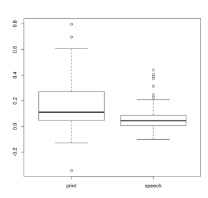
Showing us that our conditions significantly differ.  Next we want to plot this, which can be done using either base graphics:

boxplot( thedata$L_MFG_Anterior ~ thedata$condition )

base_boxplot

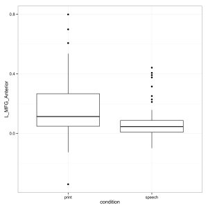
Or my preference using ggplot.

library(ggplot2)
ggplot(thedata, aes(condition, L_MFG_Anterior)) + geom_boxplot() + theme_bw()

gg_demo3

Stay tuned for extending this to multiple ROIs and other plot types.

Dealing with transforms in AFNI (Part 1)

AFNI’s main tool for dealing with transforms is cat_matvec, but in many cases you may not need to use it!  Everyone knows that transform matrices are confusing — I’ll do a post later on just covering them — but for now, I think we can all agree that it’s a relief anytime you don’t have to deal with figuring out transform matrices!

If you want to align your anatomic dataset and your EPI or DWI/DTI, you could use a range of tools like 3dWarpDrive (12-parameter affine), 3dAllineate (also 12-parameter but with more cost functions), or you could (and probably should) turn to the super-script align_epi_anat.py.  This script can do a lot!  It can do time shifting (sinc interp), motion correction, and volume co-registration with a host of available cost functions.  The added bonus of this script is that it can concatenate the transforms for you and reduce the number of times that your dataset gets warped (and thus interpolated, and therefore introduced more distortion/blur).  My “goto” call is something like this:

align_epi_anat.py -anat anat+orig -epi epi+orig -epi_base 0 -epi2anat

This will take care of Skull stripping the anatomic (and EPI), time shifting, motion correction, and volume registering the EPI to the anatomical.  I don’t mention it, but it will also take care of deobliquing the data.  If you use afni_proc.py, it will do something similar but turn off time shifting and motion correction because these are handled in their own steps.

If you wanted to combine the EPI–>ANAT and ANAT–>MNI (or TT) transform, you could run @auto_tlrc first and feed the TLRC dataset to the script:

@auto_tlrc -base TT_N27+tlrc -input anat+orig 
align_epi_anat.py -anat anat+orig -epi epi+orig -epi_base 0 -tlrc_apar anat+tlrc

In general, it’s usually a good idea to run @Align_Centers on your datasets first.  It’s not a deal-breaker, but can make your registration process less tedious.  Let’s assume our anatomic dataset is called anat+orig and our EPI is called epi+orig.

@Align_Centers -base anat+orig -dset epi+orig

This will create a new version of your EPI dataset called epi_shft+orig and introduce a transform called eli_shft.1D.  If we want to include this in our align_epi_anat.py function call, we can add this transform to our call using the “-pre_matrix” flag.  However, since by default align_epi_anat moves the anatomic to match the EPI, and we’ve reversed that AND we’ve moved the EPI to match our anatomical, we need to invert the transform before we use it.  We do that via cat_matvec (I know I said it’s nice to avoid, but sometimes we can’t!)

cat_matvec epi_shft.1D -I > inverted_transform.1D
@auto_tlrc -base TT_N27+tlrc -input anat+orig 
align_epi_anat.py -anat anat+orig -epi epi+orig -epi_base 0 \
-epi2anat \
-tlrc_apar anat+tlrc \
-pre_matrix inverted_transform.1D

Many of these concepts can be used for DWI/DTI data as well.  I’ve posted a bit on this before (and here), but I’ll try to update it again soon!