First let me say that I am a huge huge fan of Freesurfer.  It makes my life easier in so many ways by 1) creating surfaces that we can display fMRI results on; 2) giving beautiful cortical and subcortical segmentations for use in the upcoming (soon, really) pediatric Atlas that I’ve been working on; 3) useful for measures of brain volume and cortical thickness.  If I had two small complaints about Freesurfer, it’s exactly what you would expect: It’s slow (24-hours per subject on my SUPER Mac) and the Group Analysis tools aren’t always easy to interact with.

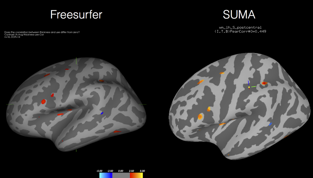
Well I’ve posted previously about how to run Freesurfer jobs in parallel so that if you have an 8-core Mac you can process 8 subjects simultaneously.  Today I’m going to show you how you can use AFNI’s tools, like 3dttest++, to get the same information out of cortical thickness measures as you do using the Freesurfer tools!  That’s right, by the end you will see how the two softwares give you identical results like these (forgive the tilt and colors being a bit off):

Let’s start by saying you obviously need AFNI and Freesurfer installed on your system.  I also find it very useful to make a SUMA folder for your fsaverage subject.  This will come in handy later for visualizing the results in SUMA:

cd $SUBJECTS_DIR/fsaverage
@SUMA_Make_Spec_FS -sid fsaverage

You’ll also need to process all of your participants through the Freesurfer pipeline, preferably with the -qcache option added onto the end:

cd /path/to/subjects/datafiles
for aSubject in Subject01 Subject02 Subject03
do
    recon-all -s $aSubject -i $aSubject/inputNifti.nii.gz -all -qcache
done

Of course you can batch these using Parallel if you want to speed things up.  Once you complete all of the processing, you will find that each subject has their Surface data stored in the aptly named ‘surf’ folder.  If you are doing cortical thickness measurements, you’ll want to locate the lh.thickness and rh.thickness files, which are the unsmoothed thickness measurements.  If you used @SUMA_Make_Spec, these are converted to GIFTI datasets by the script, and of course there are the std.141.?h.thickness.niml.dset files representing the standard mesh, again without any blurring.

At this point you have a choice, you can use AFNI/SUMA’s SurfSmooth to smooth your thickness files, or you can instead locate the files that Freesurfer has been kind enough to both resample to the fsaverage brain with different levels of smoothness and use those instead!  Those files are called lh.thickness.fwhm10.fsaverage.mgh and rh.thickness.fwhm10.fsaverage (where fwhm ranges from 0 to 25 in increments of 5).  If we want to convert these to GIFTI datasets that AFNI/SUMA can use, we simply need to use a built in Freesurfer tool (the same one used by @SUMA_Make_Spec_FS) to convert the files, called mris_convert.

mris_convert -c ./Subject01/surf/lh.thickness.fwhm10.fsaverage.mgh \
$SUBJECTS_DIR/fsaverage/surf/lh.white \
Subject01.lh.thickness.fsaverage.gii

If you do this for each hemisphere and each subject, you will end up with a folder full of thickness files already smoothed to some FWHM. You can then use ANY of the AFNI tools to perform group analysis!

3dttest++ -prefix lh.Group1_vs_Group2.gii  \
-setA Group1/*.lh*.gii \
-setB Group2/*.lh*.gii

You can then view the results in SUMA:

suma -spec /usr/local/freesurfer/subjects/fsaverage/SUMA/fsaverage_lh.spec

And then load up the surface controller and Load Dset for the output of your t-test, correlation, mixed model, the sky is the limit.  And as you can see from the above figure, the results coming out of AFNI’s tools are nearly identical to those processed directly in Freesurfer’s mri_glmfit (or qdec).

If you’re wondering why you might want to go through this effort to get identical output, beyond just the ease of using AFNI tools and the speed improvement, I’ll remind you that you can use any AFNI tool now with your Freesurfer data including 3dMVM and 3dLME!

In the past I’ve shown how to use 3dttest++ to do one-sample, paired, and two-sample t-tests for whole-brain maps in AFNI.  Occasionally there is an instance where you want to quickly generate a series of t-tests for all participants at once.  Most people (including me until recently) would simply loop over their gen_group_command.py script several times (with different sub-brick inputs each time) to accomplish this.  Another option is to use both the “short form” and the -brickwise option for 3dttest++.  The great thing about the short-form is that you can use wildcards.  So if you have every datafile in the same directory, you can do something like this:

3dttest++ -prefix all_t -brickwise -setA Subject??.stats+tlrc.HEAD

Which will conduct one t-test for every sub-brick in your input datasets.  Which of course means that you need to 1) have all of your input datasets the same size (# sub-bricks) and 2) only include conditions of interest.  Both of these requirements usually mean using 3dbucket to extract only the coefficient values as so:

3dbucket -prefix Subject01.stats+tlrc FullSubject01+tlrc.HEAD[Cond1#0_Coef, Cond2#0_Coef, Cond3#0_Coef, Cond4#0_Coef]

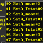
The output of the 3dttest++ with -brickwise on the datasets prepared by 3dbucket will look like the following.  You’ll notice unlabeled outputs, and one for each input sub-brick.

At this point you might want to rename your sub-bricks to easily remember what they were later, to name just the first two:

3drefit -sublabel 0 'Print_Coef' all_t+tlrc.
3drefit -sublabel 1 'Print_Tstat' all_t+tlrc.

Which results in the following newly relabeled sub-bricks.

And there you have it!  A quicker way to analyze your data without the need to loop over a script repeatedly.  Though I have to say that you should be careful because mistakes can happen and you might label something incorrectly and skew your interpretation of some results!

I don’t usually post brief updates like this, but a recent update to afni_proc.py has me really excited. As of the May 13th 2014 binaries of AFNI, you can now expect your resting state data to process considerably faster thanks to a new-ish program called 3dTproject.  3dTproject is meant to replace 3dDeconvolve for resting state processing and shows huge improvements in speed!  How fast do you ask?  What normally takes my computer (12-core Mac Pro) about an hour to process for resting state was accomplished in a mere 10 seconds using 3dTproject.

How can you get the improvements?  Update your AFNI binaries (@update.afni.binaries -d) and use afni_proc.py for your processing.  Alternatively you can call 3dTproject by hand on your data.  You’ll need to run 3dDeconvolve with with the -x1D_stop, which will setup the necessary matrices (i.e.. X.nocensor.xmat.1D) for 3dTproject to use.  Once this is done, it’s as simple as giving 3dTproject your input files, the Xmat and a censor file and you’re off to the races!

3dTproject -polort 0 -input pb04.$subj.r*.blur+tlrc.HEAD \
 -censor censor_${subj}_combined_2.1D -cenmode ZERO \
 -ort X.nocensor.xmat.1D -prefix errts.${subj}.tproject

That’s all for now!