Creating ROIs in AFNI with Coordinates

In the past, I’ve posted on creating ROIs in AFNI and ways to manipulate those ROIs once created.  But something that comes up fairly often on the AFNI message boards is how to use 3dcalc to create different ROI shapes.  The most common that I’ve found are creating spheres and cubes, I’ve made some crazy shapes lately, but for today I’m just going to cover the basics.

Creating a sphere with 3dcalc

Sphere’s have two major properties, a origin (center) and radius.  For our example, our origin will be in the left hippocampus (x=23, y=21, z=-6.5).  To create a sphere with a radius of 3mm, use the following:

3dcalc -a `@GetAfniBin`/TT_N27+tlrc.HEAD \
-prefix SphereROI \
-expr 'step(9-(x-23)*(x-23)-(y-21)*(y-21)-(z+6.5)*(z+6.5))'

Here I use the script @GetAfniBin to reference the Colin27 Template for reference so that my ROI will be in the same space, you could also use a brain in your dataset or any other template/atlas.  The first number ends up being your radius squared (3^2 = 9), followed by your coordinates.  3dcalc will treat x,y, and z in a coordinate space (and t if you want time!).  To represent positive numbers, represent them as a subtraction and to represent negative numbers in your origin, use addition.  Notice each set gets multiplied by itself.

Creating a box with 3dcalc

To define a box we simply need to define the x, y, and z coordinates that are included in our ROI.  The following code will create an ROI over part of the visual cortex.

3dcalc -LPI -a`@GetAfniBin`/TT_N27+tlrc.HEAD \ 
-prefix BoxROI \ 
-expr 'a*within(x,-12,16)*within(y,-90,-76)*within(z,4,12)'

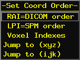
Here we tell 3dcalc that we want to use LPI (e.g. SPM) code for x,y,z, the major difference is that it it flips the X and Y, so in DICOM (or RAI) order a positive X is on the left and in LPI it’s on the right.  Similarly a positive Y would be posterior in RAI but is anterior in LPI.  You can easily use either coordinate system by using the readout in the AFNI viewer.  You can right click where it shows the x,y,z in the upper left corner and select LPI instead of RAI.

SwitchLPI

Creating ROIs from a text file with 3dUndump

If you have a series of coordinates (or just one) and you want to make a sphere quickly, you can use 3dUndump.  In 3dUndump, you specify a text file with each line representing between 3 and 5 numbers.  The first 3 (mandatory) are either xyz (coordinates) or ijk values that will represent your mask.  You set either xyz or ijk as an option to the program.  If you wish to add a value to that particular mask, you can add a fourth number, which can be useful to telling your masks apart later on!  If you use the “srad” option, you can add a fifth number to specify the radius of your ROI.

So if I had the text (mycoord.1D) file as follows:

 23 21 -6.5 1

And I executed the command:

3dUndump -master `@GetAfniBin`/TT_N27+tlrc.HEAD  -srad 4 -xyz mycoord.1D

Would create a sphere with radius 4, centered at x=23, y=21, z=-6.5 (Left Hippocampus as before), all voxels within that sphere will be set to 1.  Adding more lines to the input file will create more ROIs.   If you are using ROIs from a paper you might want to add -orient LPI.

Going beyond the basics

It’s true that you can create complex commands in 3dcalc to make even more interesting shapes (though the utility of those can be questionable).  But it’s often easier to create multiple ROIs and then use 3dcalc or 3dmask_tool to add, subtract, erode, or dilate them.  For instance if you wanted to create a circle instead of a solid sphere, you could run 3dUndump twice with two different values for srad (radius), use 3dcalc to subtract the smaller radius from the larger one and you will get the following.
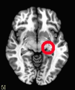
circle

An alternative approach would be to create the smaller sphere, dilate it with 3dmask_tool and then subtract the original from the dilated sphere.  The sky really is the limit, and don’t forget that you can use masks of the brain (or a specific region via whereami) to carve parts of your ROI away or add to it!
 

TORTOISE Processing of DWI/DTI (Part 2)

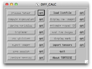
Last time, we covered how to use TORTOISE’s DIFF_PREP tool to preprocess Diffusion Weighted Images (DWI) to correct for eddy currents, motion, rotate the b-vectors (alongside the motion correction), and optionally correct b-splines if we used a T2-weighted structural image.  The next step is to use DIFF_CALC to fit tensors, inspect the results, measure ROIs, or in most of my cases, export the data to another software.  Because there are so many features, I’m only going to cover some subset in each blog post.

DIFF_CALC_1

The first thing you will notice about DIFF_CALC is that the user interface is fairly spartan looking.  Don’t be fooled, as part of TORTOISE, this application has plenty of power and is full of features.  The second thing that you may notice is there is a tiny floating window with one button for “sensitize the buttons”.  Whatever you do, don’t close that tiny floating window, it will help you recover later if you accidentally close a window without clicking “Done”.

Next you want to load your “List File”, which was generated by DIFF_PREP from the previous post.  Click “load listfile” and navigate to the directory that was created with DIFF_PREP (often ending with “_proc”).  You will see at least three possible files ending with “.list”.  To make reading this more clearly, assume that my original Diffusion image was called dwi.nii.  DIFF_PREP would have created a folder called dwi_proc and within that would be three lists called 1) dwi.list, 2) dwi_up.list and 3) dwi_DMC.list.  These represent the 1) original (read: uncorrected) data that was imported, 2) the original data after it was up sampled by DIFF_PREP, and 3) the up sampled data with all of the corrections (motion, eddy, and b-spline).

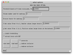
You likely want to calculate your tensors on the corrected data, so select your _DMC.list file.  Several more buttons will become available in the DIFF_CALC user interface.  I would recommend the first thing that you do is click “mask raw images”, this will specify the tensors that you will fit later only happen in the masked out brain regions.  If you click the “Opt” button next to “mask raw images”, you will see that there are some options for how you wish to apply the mask.  You can use bet (from FSL) or you can do thresholding.  Often I have excellent luck with the default settings.

Note: If you happen to close the window using the close button in the top of the window, you will notice that you’re locked out of the user interface.  Here’s where clicking the “sensitize the buttons” button will save you and restore your access to the user interface.  

tortoise_gen_mask

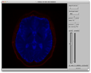
Now that a mask has been created, you can verify the mask using the “display mask” button.  This will display the window below where the mask includes regions in blue and excludes regions in red.  If the mask is not where you want it to be, go back to the mask options and try a different threshold.

tortoise_show_mask

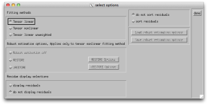
At this point, you can start to actually fit tensors!  Click the “opt” button next to “process tensors” and you will see the window below, which allows you the option of doing linear and nonlinear tensor fitting.  You can also do fits via RESTORE and iRESTORE.  For the money, the nonlinear estimation is often recommended over the linear and costs you only marginally more time for the estimation.  I also find it useful to display the residuals and to sort them!  It’s important that now that you’ve setup the options, you push the “process tensors” button on the main window.

DIFF_CALC_FIT_TENSORS

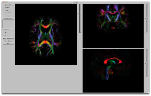
You can now view the resulting tensors (and DTI related metrics like FA) using the triplanar viewer shown below.  The viewer has an assistive panel allowing you to choose the metric that you view including the Eigen values, structural, and shown below is the DEC map that we have all come to know and love through publications.

TORTOISE_tripalne

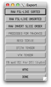
Once I view the data briefly in this viewer, I usually take the estimated tensors and export them for use in AFNI using the dialogue below:

TORTOISE_Export

But you can also export them for use with TrackVis and other formats.  The AFNI export sends out NIFTI files that go into your _proc directory (in my case dwi_proc), and can be found in a sub-folder.  The AFNI export is already named correctly for use with the tractography programs (e.g. 3dProbTrackID), which will be the topic of an upcoming post.

TORTOISE Processing of DWI/DTI (Part 1)

These instructions are for an older version of TORTOISE, if you would like to read new instructions checkout the updated tutorial HERE!

There are many options when deciding how to process Diffusion Weighted Images (DWI) and turn them into Diffusion Tensor Images (DTI).  I’ve written before about preprocessing in FSL (Part 1, Part 2) and AFNI (Part 1, Part 2), highlighting that most recommend doing some kind of eddy current “correction”, rotating the b-vectors to adjust for motion in the scanner, and often registering the data to an individuals brain.  But the capabilities are often spanning different software packages or not completely handled by the tools forcing you to write your own code to handle bvec rotation or coregistration.  Don’t get me wrong, I usually enjoy this!  But there is something to be said about using a canned software package that takes care of all of the preprocessing steps!

Enter TORTOISE (Tolerably Obsessive Registration and Tensor Optimization Indolent Software Ensemble).  TORTOISE can handle all of the preprocessing of your DWI data with full support of eddy and motion correction, BSpline correction, rotation of b-vectors, and co-registration to a structural image.  TORTOISE can also fit the tensors using both a linear fit (similar to FSL), nonlinear fit, and weighted non-linear methods (e.g. RESTORE and iRESTORE).  In this post I’ll go over the preprocessing of DWI images (DIFF_PREP) and next time I’ll go into more depth on the calculations via DIFF_CALC.  The recommendations I make are based on both the written manual (accessible on their wiki) and my own personal experience using TORTOISE.  I highly recommend using TORTOISE, which requires no additional software.  If you have a copy of IDL on your computer (or are willing to buy a copy), TORTOISE will run faster by parallelizing many of it’s operations.

Preprocessing DWI Data with DIFF_PREP 

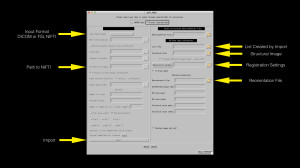
The first thing to do is get your data into TORTOISE.  You can import a variety of data formats (Phillips PAR/REC, DICOM, NIFTI, and Bruker).  I highly recommend importing from either DICOM or FSL NIFTI.  If you choose DICOM, you will need to supply TORTOISE with your gradient file, as it will not read the directions from your DICOM headers.  If you choose FSL NIFTI, TORTOISE will read your bvec and bval files from text, they just need to have the name (bvec or bval) in the filename and be in the same folder as the NIFTI file.  TORTOISE will search sub-folders for these files, so if you have multiple bvec or bval files in your folder or sub-folders, it will give you an error that it found multiple bvec/bval files and you’ll have to tidy up your file structure.

TORTOISE.001

In the image above (click to make bigger), you can see the common settings highlighted with yellow arrows.  On the import side, you’ll want to specify your format (FSL NIFTI is my recommendation), the file path to your NIFTI file (note – uncompressed NIFTI only -.nii not .nii.gz – as of this post), and then click import.  Using NIFTI files imported from dcm2nii and DIMON have worked well for me.  The one advantage to dcm2nii is that it will automatically create the bval and bvec files in the correct format for TORTOISE.

After you import the data, you will see the right side of the window becomes enabled and will automatically file in your List File location.  If you have a T2-weighted image with fat suppression, you should supply that as your Structural File.  This structural file should be skull stripped and optionally put into AC-PC alignment.  If you don’t have a T2-weighted image, you will want to turn off the BSpline correction step.  I’ve found that you can use a T1-weighted image for as Structural File so long as you don’t use BSpline correction.  If you don’t supply it a Structural Image, TORTOISE appears to make one from the B0 image.  The bottom line is that in this particular software – having a T2-weighted image for correction is very helpful.

If you have a high-resolution T1-weighted image that you wish the DWI images to be in alignment with, you can supply a Reorientation File as well.  This could be your skull-stripped anatomical image from an AFNI or FSL pipeline in the desired final orientation (e.g. RAI).  It could also be a template (e.g. MNI152).  It’s worth noting that TORTOISE is using a standard linear (“affine”) transform, which may not be as good as a non-linear transform.  But has the advantage of being part of a transform chain that only interpolates your data once!

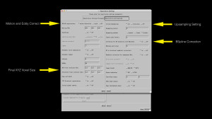
Next you’re going to click the “Registration param” button to setup the more advanced settings.

TORTOISE.002Inside your Registration Settings, I highly recommend you keep most of the defaults.  The things that I’ve found reason to change (in TORTOISE version 2.0.1) are the final DWI voxelsize resolution, it defaults to 1.5mm^3, but it may not make sense to go to such a fine grid if you collect at say 3mm^3.  The other thing that I’ve changed is the initial upsampling setting, if you have a particularly thick slice DWI image, you might consider changing it to slice_only.  In the registration settings is also where you will turn off the BSpline correction if you aren’t using a T2-weighted image with fat suppression for your structural image.

Once you click “Apply”, TORTOISE will start working.  It can take a while, so be patient.  Some windows will popup to show the registration of each direction to the B0 image and the registration of the B0 to the structural image.

Why use TORTOISE?

If you’re still reading, you might be saying to yourself “Why would I add another software package to my existing pipeline?”  Well that’s a fair question and one that I asked repeatedly, until I saw a demonstration by Paul Taylor (author of many of the AFNI tractography programs) showing the difference in tractography with and without TORTOISE processing, the presentation can be seen here, see slide 52.

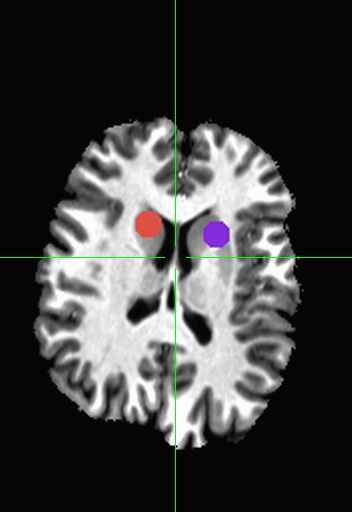
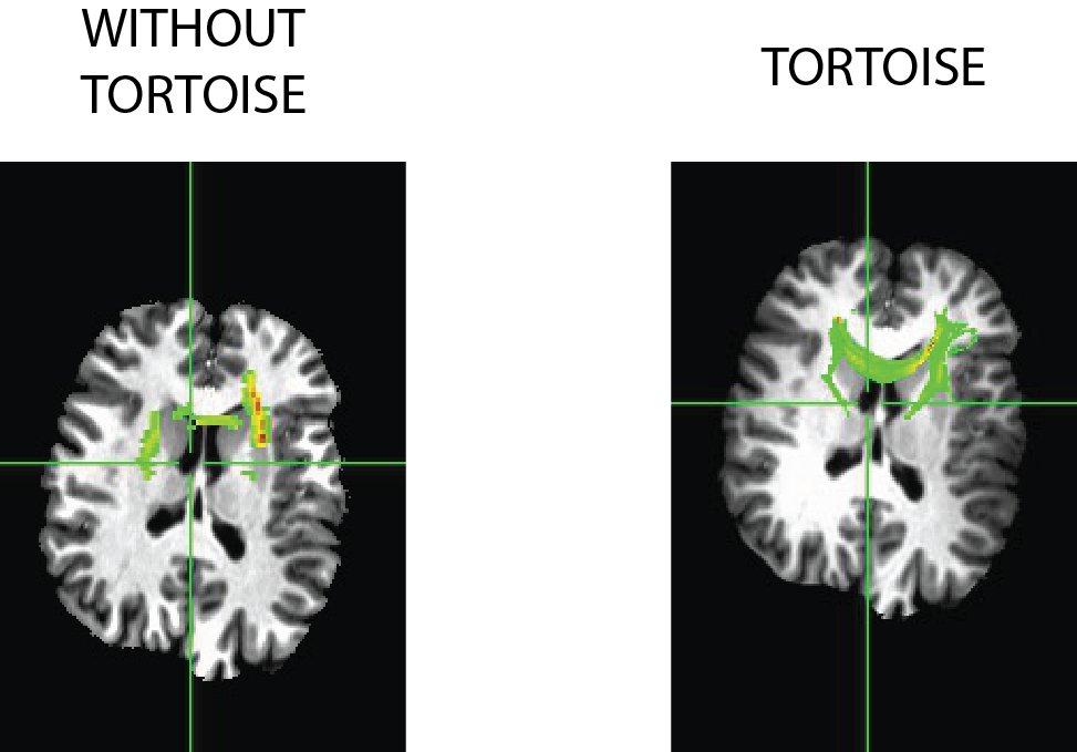
I went ahead and made a quick “off the cuff” comparison of using TORTOISE vs. only doing eddy correction (via FSL’s eddy_correct) tool.   This sample with TORTOISE uses all of the default and suggested options listed above, but without a T2-weight structural image (I didn’t have one).  TORTOISE rotated the bvecs automatically, but I did not rotate the bvecs on the FSL pipeline, though there was relatively little movement, so I wouldn’t expect the rotation to make a big difference.  Tensors were fit via a linear fit method and then deterministic tractography was used (LOGIC: AND) between two frontal ROIs shown below:

ROIs

There are plenty of fibers that appear in the NON-TORTOISE output, but considerably more connections in the TORTOISE output.  It appears that the fibers are partially going through the ventricles, this is mostly an illusion based on the slice and viewing direction, the tract in reality (mostly) goes around the ventricle.

TORTOISE_DEMO

Stay tuned for the tensor fitting segment via TORTOISE (DIFF_CALC).  I will also get around to describing how you can use TORTOISE with your AFNI processing pipeline.

Year 1 Reflection

I really started investing in this blog in November 2012.  In the first month it received 12 hits.  In the second month, it also received 12 hits.  But as we’ve added more content over the past year, the number of hits has continued to go up.  And I’m very happy that today, we celebrate more than 4500 visitors!

It’s also been a wonderful learning experience on my end, I’ve started mixing posts of different lengths and breaking things into series.  The plus side of this is that more content gets up quickly.  The downside is that content can be harder to find, so I thought in addition to patting myself on the back, I could use this post to present in a more organized manner all of the posts over the past year.

DTI

Basics of DTI Analysis in FSL

Analyzing DTI data in AFNI (Part 1)

Analyzing DTI data in AFNI (Part 2)

Rotating bvecs for DTI fitting

fMRI – File Conversions

Converting DICOM to NIFTI

The mysterious flipped brain

fMRI – Single Subject

Installing AFNI’s uber_subject.py

Single subject analysis in AFNI (uber_subject.py)

Using afni_proc.py for (Single Subject) fMRI Analysis

Using multiple basis functions in afni_proc.py

Statistics on the Brain with AFNI

fMRI – Group Analysis

Basics of AFNI Group Analysis (Part 1)

Basics of AFNI Group Analysis (Part 2)

Correlating Brain & Behavior in AFNI

fMRI – Region of Interest / Masks

Creating Volume ROIs in AFNI

Fun with AFNI Masks

Quickly Creating Masks in AFNI

fMRI – Other

Connectivity Analysis in AFNI (Part 1)

Displaying fMRI Results on Surfaces with SUMA

Simulating fMRI Designs

Adjusting smoothness for multi-scanner comparisons

Creating automated QA Snapshots

Creating AFNI images from command-line with Xvfb

Quality Checking fMRI Data

Parallelizing Freesurfer

Write your own fMRI programs using AFNI API (Part 1)

EEG/ERP

EEG Processing Tools

Source code for EEG Processing Tools

Preprocessing EEG Data

Installing ERP PCA Toolkit

Analyzing ERP Data with PCA-ANOVA in R

Finding ERP Noise Outliers

General Computing

The power of doing things in Parallel

Using GSL with Xcode

Tips for Remote Processing

The future

I will continue to update the blog with new information as it becomes available (or I learn it).  For having grown up on EEG/ERP, I realize the blog is light in this content and have a series of posts in draft to address this issue.  Further, I intend to start writing more posts on using R, statistics, and general computation.

It is also my hope that the team of bloggers here at CogNeuroStats will begin to grow.  I’ve talked to a few interested individuals and have some leads on contributors.  If you’re interested, drop me a line: peter (at) cogneurostats.com

Statistics on the Brain with AFNI

In previous posts I’ve covered how to use AFNI to run GLMs on your data to find task-related activations.  But there are a host of other statistics that you can run on the brain outside of the GLM!  And this is where AFNI really shines in terms of having a diverse set of tools, yet can be confusing because there are so many tools.  So here’s some basics:

Whole-Brain Statistics

To calculate the statistics (e.g. mean, standard deviation, sum) for a whole brain you have a few options.

3dMean – will calculate a dataset consisting of Mean, Std. Deviation, or Square Root of your input datasets.  This can be very useful if you want to create an “Average Brain” or for calculations to make a z-score of your input datasets.

3dMean -prefix AverageBrain brain1.nii.gz brain2.nii.gz brain3.nii.gz

3dcalc – is the general purpose calculator for whole-brain images.  It can do every type of mathematical calculation imaginable on images (e.g. multiplication) as well as perform conjunction style conditioning (e.g. AND, OR).

3dcalc -a 'Dataset1+tlrc.' -b 'Dataset2+tlrc.' -prefix both -expr 'AND(a,b)'

Statistics over Time

AFNI tools that work over Time or multiple sub-bricks of a dataset have a capital T in the name.

3dTstat – this tool calculates statistics over time.  If you wish to find the average for each voxel over a time series of the first 201 time points in a data file.

3dTstat -prefix AvgOverTime -mean InputDset[0..200]

Statistics within an image

If instead of calculating statistics at each voxel, you can calculate a statistic (e.g. Mean) over the entire image – so that you get one number for an image.  There’s a tool for that.

3dBrickStat – this tool calculates statistics over a single image.  You can also pass it multiple images using sub-brick selectors.

3dBrickStat -mean -mask ../TT_Mask_small+tlrc.HEAD $aSub[1]

The code above calculates the mean of all voxels in the mask and returns one number.

Using calculated numbers inside or your scripts

ccalc – Is a useful general calculation tool.  It behaves like 3dcalc / 1deval.

var=`3dBrickStat -var -mask ../TT_Mask_small+tlrc.HEAD $aSub[1]`
std=`ccalc -expr "sqrt($var)"`

Using the example above, I calculate variance from a dataset (masking outside of the brain) and then get  the standard deviation using ccalc.